
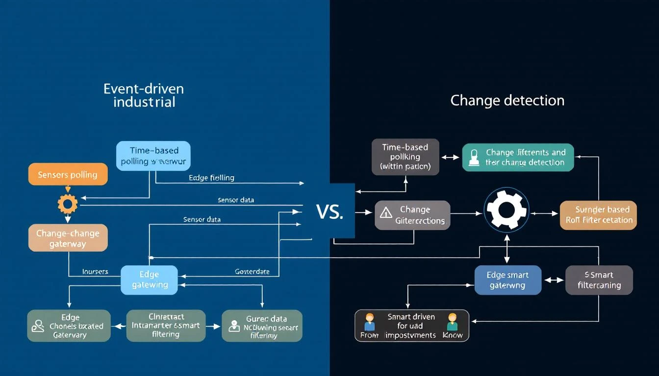
Event-Driven Tag Delivery in IIoT: Why Polling Everything at Fixed Intervals Is Wasting Your Bandwidth [2026]

· 11 min read

Event-Driven Tag Detection

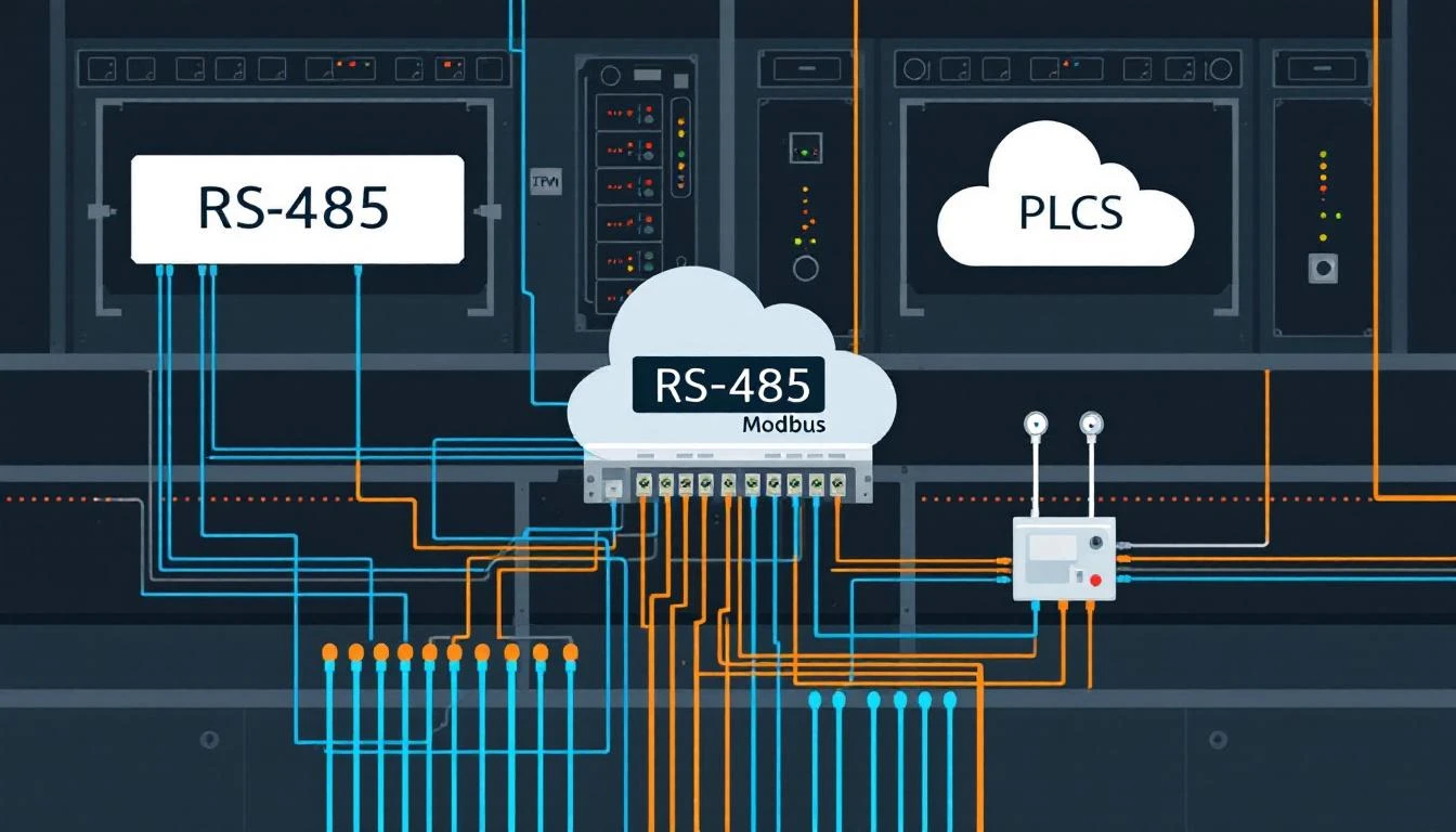
Most IIoT deployments start the same way: poll every PLC register every second, serialize all values to JSON, and push everything to the cloud over MQTT. It works — until your cellular data bill arrives, or your broker starts choking on 500,000 messages per day from a single gateway, or you realize that 95% of those messages contain values that haven't changed since the last read.

The reality of industrial data is that most values don't change most of the time. A chiller's tank temperature drifts by a fraction of a degree per minute. A blender's motor state is "running" for 8 hours straight. A conveyor's alarm register reads zero all day — until the instant it doesn't, and that instant matters more than the previous 86,400 identical readings.

This guide covers a smarter approach: event-driven tag delivery, where the edge gateway reads at regular intervals but only transmits when something actually changes — and when something does change, it can trigger reads of related tags for complete context.

The Problem with Fixed-Interval Everything

Let's quantify the waste. Consider a typical industrial chiller with 10 compressor circuits, each exposing 16 process tags (temperatures, pressures, flow rates) and 3 alarm registers:

Tags per circuit:  16 process + 3 alarm = 19 tags
Total tags: 10 circuits × 19 = 190 tags
Poll interval: All at 1 second

At JSON format with timestamp, tag ID, and value, each data point is roughly 50 bytes. Per second, that's:

190 tags × 50 bytes = 9,500 bytes/second
= 570 KB/minute
= 34.2 MB/hour
= 821 MB/day

Over a cellular connection at $5/GB, that's $4.10/day per chiller — just for data that's overwhelmingly identical to what was sent one second ago.

Now let's separate the tags by their actual change frequency:

Tag TypeCountActual Change Frequency% of Total Data
Process temperatures100Every 30-60 seconds52.6%
Process pressures50Every 10-30 seconds26.3%
Flow rates10Every 5-15 seconds5.3%
Alarm bits30~1-5 times per day15.8%

Those 30 alarm registers — 15.8% of your data volume — change roughly 5 times per day. You're transmitting them 86,400 times. That's a 17,280x overhead on alarm data.

The Three Pillars of Event-Driven Delivery

A well-designed edge gateway implements three complementary strategies:

1. Compare-on-Read (Change Detection)

The simplest optimization: after reading a tag value from the PLC, compare it against the last transmitted value. If it hasn't changed, don't send it.

The implementation is straightforward:

# Pseudocode — NOT from any specific codebase
def should_deliver(tag, new_value, new_status):
# Always deliver the first reading
if not tag.has_been_read:
return True

# Always deliver on status change (device went offline/online)
if tag.last_status != new_status:
return True

# Compare values if compare flag is enabled
if tag.compare_enabled:
if tag.last_value != new_value:
return True
return False # Value unchanged, skip

# If compare disabled, always deliver
return True

Which tags should use change detection?

  • Alarm/status registers: Always. These are event-driven by nature — you need the transitions, not the steady state.
  • Digital I/O: Always. Binary values either changed or they didn't.
  • Configuration registers: Always. Software version numbers, setpoints, and device parameters change rarely.
  • Temperatures and pressures: Situational. If the process is stable, most readings are identical. But if you need trending data for analytics, you may want periodic delivery regardless.
  • Counter registers: Never. Counters increment continuously — every reading is "different" — and you need the raw values for accurate rate calculations.

The gotcha with floating-point comparison: Comparing IEEE 754 floats for exact equality is unreliable due to rounding. For float-typed tags, use a deadband:

# Apply deadband for float comparison
def float_changed(old_val, new_val, deadband=0.1):
return abs(new_val - old_val) > deadband

A temperature deadband of 0.1°F means you'll transmit when the temperature moves meaningfully, but ignore sensor noise.

2. Dependent Tags (Contextual Reads)

Here's where event-driven delivery gets powerful. Consider this scenario:

A chiller's compressor status word is a 16-bit register where each bit represents a different state: running, loaded, alarm, lockout, etc. You poll this register every second with change detection enabled. When bit 7 flips from 0 to 1 (alarm condition), you need more than just the status word — you need the discharge pressure, suction temperature, refrigerant level, and superheat at that exact moment to diagnose the alarm.

The solution: dependent tag chains. When a parent tag's value changes, the gateway immediately triggers a forced read of all dependent tags, delivering the complete snapshot:

Parent Tag:    Compressor Status Word (polled every 1s, compare=true)
Dependent Tags:
├── Discharge Pressure (read only when status changes)
├── Suction Temperature (read only when status changes)
├── Refrigerant Liquid Temp (read only when status changes)
├── Superheat (read only when status changes)
└── Subcool (read only when status changes)

In normal operation, the gateway reads only the status word — one register per second per compressor. When the status word changes, it reads 6 registers total and delivers them as a single timestamped group. The result:

  • Steady state: 1 register/second → 50 bytes/second
  • Event triggered: 6 registers at once → 300 bytes (once, at the moment of change)
  • vs. polling everything: 6 registers/second → 300 bytes/second (continuously)

Bandwidth savings: 99.8% during steady state, with zero data loss at the moment that matters.

3. Calculated Tags (Bit-Level Decomposition)

Industrial PLCs often pack multiple boolean signals into a single 16-bit or 32-bit "status word" or "alarm word." Each bit has a specific meaning defined in the PLC program documentation:

Alarm Word (uint16):
Bit 0: High Temperature Alarm
Bit 1: Low Pressure Alarm
Bit 2: Flow Switch Fault
Bit 3: Motor Overload
Bit 4: Sensor Open Circuit
Bit 5: Communication Fault
Bits 6-15: Reserved

A naive approach reads the entire word and sends it to the cloud, leaving the bit-level parsing to the backend. A better approach: the edge gateway decomposes the word into individual boolean tags at read time.

The gateway reads the parent tag (the alarm word), and for each calculated tag, it applies a shift and mask operation to extract the individual bit:

Individual Alarm = (alarm_word >> bit_position) & mask

Each calculated tag gets its own change detection. So when Bit 2 (Flow Switch Fault) transitions from 0 to 1, the gateway transmits only that specific alarm — not the entire word, and not any unchanged bits.

Why this matters at scale: A 10-circuit chiller has 30 alarm registers (3 per circuit), each 16 bits wide. That's 480 individual alarm conditions. Without bit decomposition, a single bit flip in one register transmits all 30 registers (because the polling cycle doesn't know which register changed). With calculated tags, only the one changed boolean is transmitted.

Batching: Grouping Efficiency

Even with change detection, transmitting each changed tag as an individual MQTT message creates excessive overhead. MQTT headers, TLS framing, and TCP acknowledgments add 80-100 bytes of overhead per message. A 50-byte tag value in a 130-byte envelope is 62% overhead.

The solution: time-bounded batching. The gateway accumulates changed tag values into a batch, then transmits the batch when either:

  1. The batch reaches a size threshold (e.g., 4KB of accumulated data)
  2. A time limit expires (e.g., 10-30 seconds since the batch started collecting)

The batch structure groups values by timestamp:

{
"groups": [
{
"ts": 1709335200,
"device_type": 1018,
"serial_number": 2411001,
"values": [
{"id": 1, "values": [245]},
{"id": 6, "values": [187]},
{"id": 7, "values": [42]}
]
}
]
}

Critical exception: alarm tags bypass batching. When a status register changes, you don't want the alarm notification sitting in a batch buffer for 30 seconds. Alarm tags should be marked as do_not_batch — they're serialized and transmitted immediately as individual messages with QoS 1 delivery confirmation.

This creates a two-tier delivery system:

Data TypeDeliveryLatencyBatching
Process valuesChange-detected, batched10-30 secondsYes
Alarm/status bitsChange-detected, immediate<1 secondNo
Periodic valuesTime-based, batched10-60 secondsYes

Binary vs. JSON: The Encoding Decision

The batch payload format has a surprisingly large impact on bandwidth. Consider a batch with 50 tag values:

JSON format:

{"groups":[{"ts":1709335200,"device_type":1018,"serial_number":2411001,"values":[{"id":1,"values":[245]},{"id":2,"values":[187]},...]}]}

Typical size: 2,500-3,000 bytes for 50 values

Binary format:

Header:     1 byte  (magic byte 0xF7)
Group count: 4 bytes
Per group:
Timestamp: 4 bytes
Device type: 2 bytes
Serial number: 4 bytes
Value count: 4 bytes
Per value:
Tag ID: 2 bytes
Status: 1 byte
Value count: 1 byte
Value size: 1 byte (1=bool/int8, 2=int16, 4=int32/float)
Values: 1-4 bytes each

Typical size: 400-600 bytes for 50 values

That's a 5-7x reduction — from 3KB to ~500 bytes per batch. Over cellular, this is transformative. A device that transmits 34 MB/day in JSON drops to 5-7 MB/day in binary, before even accounting for change detection.

The trade-off: binary payloads require a schema-aware decoder on the cloud side. Both the gateway and the backend must agree on the encoding format. In practice, most production IIoT platforms use binary encoding for device-to-cloud telemetry and JSON for cloud-to-device commands (where human readability matters and message volume is low).

The Hourly Reset: Catching Drift

One subtle problem with pure change detection: if a value drifts by tiny increments — each below the comparison threshold — the cloud's cached value can slowly diverge from reality. After hours of accumulated micro-drift, the dashboard shows 72.3°F while the actual temperature is 74.1°F.

The solution: periodic forced reads. Every hour (or at another configurable interval), the gateway resets all "read once" flags and forces a complete read of every tag, delivering all current values regardless of change. This acts as a synchronization pulse that corrects any accumulated drift and confirms that all devices are still online.

The hourly reset typically generates one large batch — a snapshot of all 190 tags — adding roughly 10-15KB once per hour. That's negligible compared to the savings from change detection during the other 3,599 seconds.

Quantifying the Savings

Let's revisit our 10-circuit chiller example with event-driven delivery:

Before (fixed interval, everything at 1s):

190 tags × 86,400 seconds × 50 bytes = 821 MB/day

After (event-driven with change detection):

Process values: 160 tags × avg 2 changes/min × 1440 min × 50 bytes = 23 MB/day
Alarm bits: 30 tags × avg 5 changes/day × 50 bytes = 7.5 KB/day
Hourly resets: 190 tags × 24 resets × 50 bytes = 228 KB/day
Overhead (headers, keepalives): ≈ 2 MB/day
──────────────────────────────────────────────────────
Total: ≈ 25.2 MB/day

With binary encoding instead of JSON:

≈ 25.2 MB/day ÷ 5.5 (binary compression) ≈ 4.6 MB/day

Net reduction: 821 MB → 4.6 MB = 99.4% bandwidth savings.

On a $5/GB cellular plan, that's $4.10/day → $0.02/day per chiller.

Implementation Checklist

If you're building or evaluating an edge gateway for event-driven tag delivery, here's what to look for:

  • Per-tag compare flag — Can you enable/disable change detection per tag?
  • Per-tag polling interval — Can fast-changing and slow-changing tags have different read rates?
  • Dependent tag chains — Can a parent tag's change trigger reads of related tags?
  • Bit-level calculated tags — Can alarm words be decomposed into individual booleans?
  • Bypass batching for alarms — Are alarm tags delivered immediately, bypassing the batch buffer?
  • Binary encoding option — Can the gateway serialize in binary instead of JSON?
  • Periodic forced sync — Does the gateway do hourly (or configurable) full reads?
  • Link state tracking — Is device online/offline status treated as a first-class event?

How machineCDN Handles Event-Driven Delivery

machineCDN's edge gateway implements all of these strategies natively. Every tag in the device configuration carries its own polling interval, change detection flag, and batch/immediate delivery preference. Alarm registers are automatically configured for 1-second polling with change detection and immediate delivery. Process values use configurable intervals with batched transmission. The gateway supports both JSON and compact binary encoding, with automatic store-and-forward buffering that retains data through connectivity outages.

The result: plants running machineCDN gateways over cellular connections typically see 95-99% lower data volumes compared to naive fixed-interval polling — without losing a single alarm event or meaningful process change.


Tired of paying for the same unchanged data point 86,400 times a day? machineCDN delivers only the data that matters — alarms instantly, process values on change, with full periodic sync. See how much bandwidth you can save.

Modbus RTU Serial Link Tuning: Baud Rate, Parity, and Timeout Optimization for Reliable PLC Communication [2026]

· 11 min read

Modbus RTU Serial Communication

Modbus TCP gets all the attention in modern IIoT deployments, but Modbus RTU over RS-485 remains the workhorse of industrial communication. Millions of devices — temperature controllers, VFDs, power meters, PLCs, and process instruments — speak Modbus RTU natively. When you're building an edge gateway that bridges these devices to the cloud, getting the serial link parameters right is the difference between rock-solid telemetry and a frustrating stream of timeouts and CRC errors.

This guide covers the six critical parameters that govern Modbus RTU serial communication, the real-world trade-offs behind each one, and the tuning strategies that separate production-grade deployments from lab prototypes.

The Six Parameters That Control Everything

Every Modbus RTU serial connection is defined by six parameters that must match between the master (your gateway) and every slave device on the bus:

1. Baud Rate

The baud rate determines how many bits per second travel across the RS-485 bus. Common values:

Baud RateBits/secTypical Use Case
96009,600Legacy devices, long cable runs (>500m)
1920019,200Standard industrial default
3840038,400Mid-range, common in newer PLCs
5760057,600Higher-speed applications
115200115,200Short runs, high-frequency polling

The real-world constraint: Every device on the RS-485 bus must use the same baud rate. If you have a mix of legacy power meters at 9600 baud and newer VFDs at 38400, you need separate RS-485 segments — each with its own serial port on the gateway.

Practical recommendation: Start at 19200 baud. It's universally supported, tolerant of cable lengths up to 1000m, and fast enough for most 1-second polling cycles. Only go higher if your polling budget demands it and your cable runs are short.

2. Parity Bit

Parity provides basic error detection at the frame level:

  • Even parity (E): Most common in industrial settings. The parity bit is set so the total number of 1-bits (data + parity) is even.
  • Odd parity (O): Less common, but some older devices default to it.
  • No parity (N): Removes the parity bit entirely. When using no parity, you typically add a second stop bit to maintain frame timing.

The Modbus RTU specification recommends even parity with one stop bit as the default (8E1). However, many devices ship configured for 8N1 (no parity, one stop bit) or 8N2 (no parity, two stop bits).

Why it matters: A parity mismatch doesn't generate an error message — the slave device simply ignores the malformed frame. You'll see ETIMEDOUT errors on the master side, and the failure mode looks identical to a wiring problem or wrong slave address. This is the single most common misconfiguration in Modbus RTU deployments.

3. Data Bits

Almost universally 8 bits in modern Modbus RTU. Some ancient devices use 7-bit ASCII mode, but if you encounter one in 2026, it's time for a hardware upgrade. Don't waste time debugging 7-bit configurations — the Modbus RTU specification mandates 8 data bits.

4. Stop Bits

Stop bits mark the end of each byte frame:

  • 1 stop bit: Standard when using parity (8E1 or 8O1)
  • 2 stop bits: Standard when NOT using parity (8N2)

The total frame length should be 11 bits: 1 start + 8 data + 1 parity + 1 stop, OR 1 start + 8 data + 0 parity + 2 stop. This 11-bit frame length matters because the Modbus RTU inter-frame gap (the "silent interval" between messages) is defined as 3.5 character times — and a "character time" is 11 bits at the configured baud rate.

5. Byte Timeout

This is where things get interesting — and where most tuning guides fall short.

The byte timeout (also called "inter-character timeout" or "character timeout") defines how long the master waits between individual bytes within a single response frame. If the gap between any two consecutive bytes exceeds this timeout, the master treats it as a frame boundary.

The Modbus RTU specification says: The inter-character gap must not exceed 1.5 character times. At 9600 baud with 11-bit frames, one character time is 11/9600 = 1.146ms, so the maximum inter-character gap is 1.5 × 1.146ms ≈ 1.72ms.

What actually happens in practice:

At 9600 baud:  1 char = 1.146ms → byte timeout ≈ 2ms (safe margin)
At 19200 baud: 1 char = 0.573ms → byte timeout ≈ 1ms
At 38400 baud: 1 char = 0.286ms → byte timeout ≈ 500μs
At 115200 baud: 1 char = 0.095ms → byte timeout ≈ 200μs

The catch: At baud rates above 19200, the byte timeout drops below 1ms. Most operating systems can't guarantee sub-millisecond timer resolution, especially on embedded Linux or OpenWrt. This is why many Modbus RTU implementations clamp the byte timeout to a minimum of 500μs regardless of baud rate.

Practical recommendation: Set byte timeout to max(500μs, 2 × character_time). On embedded gateways running Linux, use 1000μs (1ms) as a safe floor.

6. Response Timeout

The response timeout defines how long the master waits after sending a request before declaring the slave unresponsive. This is the most impactful tuning parameter for overall system performance.

Factors that affect response time:

  1. Request transmission time: At 19200 baud, an 8-byte request takes ~4.6ms
  2. Slave processing time: Varies from 1ms (simple register read) to 50ms+ (complex calculations or EEPROM access)
  3. Response transmission time: At 19200 baud, a 40-register response (~85 bytes) takes ~48.7ms
  4. RS-485 transceiver turnaround: 10-50μs

The math for worst case:

Total = request_tx + slave_processing + turnaround + response_tx
= 4.6ms + 50ms + 0.05ms + 48.7ms
≈ 103ms

Practical recommendation: Set response timeout to 200-500ms for most applications. Some slow devices (energy meters doing power quality calculations) may need 1000ms. If you're polling temperature sensors that update once per second, there's no penalty to a generous 500ms timeout.

The retry question: When a timeout occurs, should you retry immediately? In production edge gateways, the answer is nuanced:

  • Retry 2-3 times before marking the device as offline
  • Insert a 50ms pause between retries to let the bus settle
  • Flush the serial buffer between retries to clear any partial frames
  • Track consecutive timeouts — if a device fails 3 reads in a row, something has changed (wiring, device failure, address conflict)

RS-485 Bus Topology: The Physical Foundation

No amount of parameter tuning can compensate for bad RS-485 wiring. The critical rules:

Daisy-chain only. RS-485 is a multi-drop bus, NOT a star topology. Every device must be wired in series — A to A, B to B — from the first device to the last.

Gateway ---[A/B]--- Device1 ---[A/B]--- Device2 ---[A/B]--- Device3
|
120Ω terminator

Termination resistors: Place a 120Ω resistor across A and B at both ends of the bus — at the gateway and at the last device. Without termination, reflections on long cable runs cause bit errors that look like random CRC failures.

Cable length limits:

Baud RateMax Cable Length
96001200m (3900 ft)
192001000m (3200 ft)
38400700m (2300 ft)
115200300m (1000 ft)

Maximum devices per segment: The RS-485 spec allows 32 unit loads per segment. Modern 1/4 unit-load transceivers can push this to 128, but in practice, keep it under 32 devices to maintain signal integrity.

Slave Address Configuration

Every device on a Modbus RTU bus needs a unique slave address (1-247). Address 0 is broadcast-only (no response expected), and addresses 248-255 are reserved.

The slave address is configured at the device level — typically through DIP switches, front-panel menus, or configuration software. The gateway needs to match.

Common mistake: Address 1 is the factory default for almost every Modbus device. If you connect two new devices without changing addresses, neither will respond reliably — they'll both try to drive the bus simultaneously, corrupting each other's responses.

Contiguous Register Grouping: The Bandwidth Multiplier

The most impactful optimization for Modbus RTU polling performance isn't a link parameter — it's how you structure your read requests.

Modbus function codes 03 (Read Holding Registers) and 04 (Read Input Registers) can read up to 125 contiguous registers in a single request. Instead of issuing separate requests for each tag, a well-designed gateway groups tags by:

  1. Function code — holding registers and input registers require different commands
  2. Address contiguity — registers must be adjacent (no gaps)
  3. Polling interval — tags polled at the same rate should be read together
  4. Maximum PDU size — cap at 50-100 registers per request to avoid overwhelming slow devices

Example: If you need registers 40001, 40002, 40003, 40010, 40011:

  • Naive approach: 5 separate read requests (5 × 12ms round-trip = 60ms)
  • Grouped approach: Read 40001-40003 in one request, 40010-40011 in another (2 × 12ms = 24ms)

The gap between 40003 and 40010 breaks contiguity, so two requests are optimal. But reading 40001-40011 as one block (11 registers) might be acceptable — the extra 7 "wasted" registers add only ~7ms of transmission time, which is less than the overhead of an additional request-response cycle.

Production-grade gateways build contiguous read groups at startup and maintain them throughout the polling cycle, only splitting groups when address gaps exceed a configurable threshold.

Error Handling: Beyond the CRC

Modbus RTU includes a 16-bit CRC at the end of every frame. If the CRC doesn't match, the frame is discarded. But there are several failure modes beyond CRC errors:

ETIMEDOUT — No response from slave:

  • Wrong slave address
  • Baud rate or parity mismatch
  • Wiring fault (A/B swapped, broken connection)
  • Device powered off or in bootloader mode
  • Bus contention (two devices with same address)

ECONNRESET — Connection reset:

  • On RS-485, this usually means the serial port driver detected a framing error
  • Often caused by electrical noise or ground loops
  • Add ferrite cores to cables near VFDs and motor drives

EBADF — Bad file descriptor:

  • The serial port was disconnected (USB-to-RS485 adapter unplugged)
  • Requires closing and reopening the serial connection

EPIPE — Broken pipe:

  • Rare on physical serial ports, more common on virtual serial ports or serial-over-TCP bridges
  • Indicates the underlying transport has failed

For each of these errors, a robust gateway should:

  1. Close the Modbus connection and flush all buffers
  2. Wait a brief cooldown (100-500ms) before attempting reconnection
  3. Update link state to notify the cloud that the device is offline
  4. Log the error type for remote diagnostics

Tuning for Specific Device Types

Different industrial devices have different Modbus RTU characteristics:

Temperature Controllers (TCUs)

  • Typically use function code 03 (holding registers)
  • Response times: 5-15ms
  • Recommended timeout: 200ms
  • Polling interval: 5-60 seconds (temperatures change slowly)

Variable Frequency Drives (VFDs)

  • Often have non-contiguous register maps
  • Response times: 10-30ms
  • Recommended timeout: 300ms
  • Polling interval: 1-5 seconds for speed/current, 60s for configuration

Power/Energy Meters

  • Large register blocks (power quality data)
  • Response times: 20-100ms (some meters buffer internally)
  • Recommended timeout: 500-1000ms
  • Polling interval: 1-15 seconds depending on resolution needed

Central Chillers (Multi-Circuit)

  • Dozens of input registers per compressor circuit
  • Deep register maps spanning 700+ addresses
  • Naturally contiguous register layouts within each circuit
  • Alarm bit registers should be polled at 1-second intervals with change detection
  • Process values (temperatures, pressures) can use 60-second intervals

Putting It All Together

A production Modbus RTU configuration for a typical industrial gateway looks like this:

# Example configuration (generic format)
serial_port: /dev/ttyUSB0
baud_rate: 19200
parity: even # 'E' — matches Modbus spec default
data_bits: 8
stop_bits: 1
slave_address: 1
byte_timeout_ms: 1
response_timeout_ms: 300

# Polling strategy
max_registers_per_read: 50
retry_count: 3
retry_delay_ms: 50
flush_between_retries: true

How machineCDN Handles Modbus RTU

machineCDN's edge gateway handles both Modbus TCP and Modbus RTU through a unified data acquisition layer. The gateway auto-configures serial link parameters from the device profile, groups contiguous registers for optimal bus utilization, implements intelligent retry logic with bus-level error recovery, and bridges Modbus RTU data to cloud-bound MQTT with store-and-forward buffering. Whether your devices speak Modbus RTU at 9600 baud or EtherNet/IP over Gigabit Ethernet, the data arrives in the same normalized format — ready for analytics, alerting, and operational dashboards.


Need to connect legacy Modbus RTU devices to a modern IIoT platform? machineCDN bridges serial protocols to the cloud without replacing your existing equipment. Talk to us about your multi-protocol deployment.

Best Alarm Management Software for Manufacturing in 2026: Reduce Noise, Catch Real Problems

· 9 min read
MachineCDN Team
Industrial IoT Experts

The average manufacturing plant generates thousands of alarms per day. Most operators ignore them. Not because they're lazy — because they've learned from experience that 90% of alarms are noise. Nuisance alarms. Standing alarms. Alarm floods during startup sequences. The sheer volume has trained operators to dismiss alerts that might actually matter.

This is the alarm management crisis in manufacturing, and it kills people, destroys equipment, and costs billions annually. The ISA-18.2 standard for alarm management exists precisely because poor alarm practices have been linked to major industrial incidents worldwide.

The good news: modern IIoT platforms are finally giving manufacturers the tools to rationalize, prioritize, and manage alarms effectively — if you pick the right one.

Augury Pricing in 2026: What Does Augury Actually Cost?

· 7 min read
MachineCDN Team
Industrial IoT Experts

If you've been evaluating vibration monitoring and machine health platforms, Augury's name has probably come up. Their sensor-based approach to predictive maintenance has earned attention from manufacturers across food & beverage, chemicals, and consumer goods.

But when it comes to pricing, Augury follows the same playbook as most enterprise IIoT vendors: no public pricing, mandatory sales calls, and quotes that vary wildly based on how many machines you're monitoring.

Let's break down what Augury actually costs in 2026 — based on publicly available information, industry analyst reports, and what manufacturing engineers report paying.

Binary Payload Encoding for Industrial MQTT: Cutting Bandwidth by 10x on Constrained Networks [2026]

· 13 min read

Binary Payload Encoding

JSON is killing your cellular data budget.

When your edge gateway publishes a single temperature reading as {"tag_id": 42, "value": 23.45, "type": "float", "status": 0, "ts": 1709312400}, that's 72 bytes of text to convey 10 bytes of actual information: a 2-byte tag ID, a 4-byte float, a 1-byte status code, and a 4-byte timestamp (which is shared across all tags in the same poll cycle anyway).

At 200 tags polled every 5 seconds, JSON payloads consume roughly 100 KB/minute — over 4 GB/month. On a $15/month cellular plan with a 1 GB cap, you've blown your data budget by day 8.

Binary encoding solves this. By designing a compact wire format purpose-built for industrial telemetry, you can reduce per-tag overhead from ~70 bytes to ~7 bytes — a 10x reduction that makes cellular and satellite IIoT deployments economically viable.

This article covers the engineering of binary payload formats for industrial MQTT, from byte-level encoding decisions to the buffering and delivery systems that ensure data integrity.

Why JSON Falls Short for Industrial Telemetry

JSON became the default payload format for MQTT in the IIoT world because it's human-readable, self-describing, and every platform can parse it. These are real advantages during development and debugging. But they come at a cost that compounds brutally at scale.

The Overhead Tax

Let's dissect a typical JSON telemetry message:

{
"device_type": 1010,
"serial": 1106550353,
"ts": 1709312400,
"tags": [
{"id": 1, "status": 0, "type": "uint16", "values": [4200]},
{"id": 2, "status": 0, "type": "float", "values": [23.45]},
{"id": 3, "status": 0, "type": "bool", "values": [1]}
]
}

This payload is approximately 250 bytes. The actual data content:

  • Device type: 2 bytes
  • Serial number: 4 bytes
  • Timestamp: 4 bytes
  • 3 tag values: 2 + 4 + 1 = 7 bytes
  • 3 tag IDs: 6 bytes
  • 3 status codes: 3 bytes

Total useful data: 26 bytes. The other 224 bytes are structural overhead — curly braces, square brackets, quotation marks, colons, commas, key names, and redundant type strings.

That's an overhead ratio of 9.6x. For every byte of machine data, you're transmitting nearly 10 bytes of JSON syntax.

CPU Cost on Embedded Gateways

JSON serialization isn't free on embedded hardware. Constructing JSON objects, converting numbers to strings, escaping special characters, and computing string lengths all consume CPU cycles that could be spent polling more tags or running edge analytics.

On an ARM Cortex-A7 gateway (common in industrial routers), JSON serialization of a 200-tag batch takes 2–5ms. The equivalent binary encoding takes 200–500μs — an order of magnitude faster. When you're polling Modbus every second and need to leave CPU headroom for other tasks, this matters.

Designing a Binary Telemetry Format

A practical binary format for industrial MQTT must balance compactness with extensibility. Here's a proven structure used in production industrial gateways.

Message Structure

┌─────────────────────────────────────────┐
│ Header │
│ ├─ Timestamp (4 bytes, uint32) │
│ ├─ Device Type (2 bytes, uint16) │
│ └─ Serial Number (4 bytes, uint32) │
├─────────────────────────────────────────┤
│ Tag Group │
│ ├─ Tag Count (2 bytes, uint16) │
│ ├─ Tag Record 1 │
│ │ ├─ Tag ID (2 bytes, uint16) │
│ │ ├─ Status (1 byte, uint8) │
│ │ ├─ Type (1 byte, uint8) │
│ │ ├─ Value Count (1 byte, uint8) │
│ │ └─ Values (variable) │
│ ├─ Tag Record 2 │
│ │ └─ ... │
│ └─ Tag Record N │
└─────────────────────────────────────────┘

Type Encoding

Use a single byte to encode the value type, which also determines the byte width of each value:

Type CodeTypeBytes per Value
0x01bool1
0x02int324
0x03uint324
0x04float324
0x05int162
0x06uint162
0x07int81
0x08uint81

This type system covers every data type you'll encounter in Modbus and EtherNet/IP PLCs. The decoder uses the type code to determine exactly how many bytes to read for each value — no parsing ambiguity, no delimiter scanning.

Size Comparison

For the same 3-tag example above:

Binary encoding:

  • Header: 10 bytes (timestamp + device type + serial)
  • Tag count: 2 bytes
  • Tag 1 (uint16): 2 + 1 + 1 + 1 + 2 = 7 bytes
  • Tag 2 (float32): 2 + 1 + 1 + 1 + 4 = 9 bytes
  • Tag 3 (bool): 2 + 1 + 1 + 1 + 1 = 6 bytes

Total: 34 bytes vs. 250 bytes for JSON. That's a 7.3x reduction.

The savings compound as tag count increases. At 100 tags (a typical mid-size PLC), a JSON batch runs 6–8 KB; the binary equivalent is 700–900 bytes. At 200 tags, JSON hits 12–16 KB while binary stays under 2 KB.

Data Grouping: Batches and Groups

Individual tag values shouldn't be published as individual MQTT messages. The MQTT protocol itself adds overhead: a PUBLISH packet includes a fixed header (2 bytes minimum), topic string (20–50 bytes for a typical industrial topic), and packet identifier (2 bytes for QoS 1). Publishing 200 individual messages means 200× this overhead.

Timestamp-Grouped Batches

The most effective grouping strategy collects all tag values from a single poll cycle into one batch, sharing a single timestamp:

[Batch Start: timestamp=1709312400]
Tag 1: id=1, status=0, type=uint16, value=4200
Tag 2: id=2, status=0, type=float, value=23.45
Tag 3: id=3, status=0, type=bool, value=1
...
[Batch End]

The timestamp in the batch header applies to all contained tags. This eliminates per-tag timestamp overhead — a savings of 4 bytes per tag, or 800 bytes across 200 tags.

Batch Size Limits

MQTT brokers and clients have maximum message size limits. Azure IoT Hub limits messages to 256 KB. AWS IoT Core allows 128 KB. Most on-premise Mosquitto deployments default to 256 MB but should be configured lower for production use.

More importantly, your edge gateway's memory and processing constraints impose practical limits. A 4 KB batch size works well for most deployments:

  • Large enough to hold 200+ tags in binary format
  • Small enough to fit in constrained gateway memory
  • Fast enough to serialize without impacting the poll loop

When a batch exceeds the configured size, close it and start a new one. The cloud decoder handles multiple batches with the same timestamp gracefully.

Change-of-Value Filtering Before Batching

Apply change-of-value (COV) filtering before adding values to the batch, not after. If a tag's value hasn't changed since the last report and COV is enabled for that tag, skip it entirely. This reduces batch sizes further during steady-state operation — when 80% of tags are unchanged, your binary batch shrinks proportionally.

However, implement a periodic full-refresh: every hour (or configurable interval), reset all COV baselines and include every tag in the next batch. This ensures the cloud always has a complete snapshot, even if individual change events were lost during a brief disconnection.

The Page Buffer: Store-and-Forward in Fixed Memory

Binary encoding solves the bandwidth problem. But you still need to handle MQTT disconnections without losing data. The page-based ring buffer is the industrial standard for store-and-forward in embedded systems.

Architecture

Pre-allocate a contiguous memory region at startup and divide it into fixed-size pages:

┌────────────────────────────────────────────────┐
│ Buffer Memory (e.g., 512 KB) │
│ │
│ ┌──────┐ ┌──────┐ ┌──────┐ ┌──────┐ ┌──────┐ │
│ │Page 0│ │Page 1│ │Page 2│ │Page 3│ │Page 4│ │
│ │ │ │ │ │ │ │ │ │ │ │
│ └──────┘ └──────┘ └──────┘ └──────┘ └──────┘ │
└────────────────────────────────────────────────┘

Pages cycle through three states:

  1. Free — empty, available for writing
  2. Work — currently being written to by the Modbus polling thread
  3. Used — full, waiting for MQTT delivery

Page Layout

Each page contains multiple messages, packed sequentially:

┌─────────────────────────────────────┐
│ Page Header (struct, ~16 bytes) │
├─────────────────────────────────────┤
│ Message 1: │
│ ├─ Message ID (4 bytes) │
│ ├─ Message Size (4 bytes) │
│ └─ Message Body (variable) │
├─────────────────────────────────────┤
│ Message 2: │
│ ├─ Message ID (4 bytes) │
│ ├─ Message Size (4 bytes) │
│ └─ Message Body (variable) │
├─────────────────────────────────────┤
│ ... (more messages) │
├─────────────────────────────────────┤
│ Free space │
└─────────────────────────────────────┘

The 4-byte message ID field is filled by the MQTT library when the message is published (at QoS 1). The gateway uses this ID to match publish acknowledgments to specific messages.

Write Path

  1. Check if the current work page has enough space for the new message (message size + 8 bytes for ID and size fields).
  2. If yes: write the message, advance the write pointer.
  3. If no: move the work page to the "used" queue, grab a free page as the new work page, and write there.
  4. If no free pages exist: grab the oldest used page (overflow condition). Log a warning — you're losing the oldest buffered data, but preserving the newest.

This overflow strategy is deliberately biased toward fresh data. In industrial monitoring, a temperature reading from 5 minutes ago is far more valuable than one from 3 days ago that was buffered during an outage.

Delivery Path

  1. Take the first page from the "used" queue.
  2. Read the next undelivered message (tracked by a per-page read pointer).
  3. Publish via MQTT at QoS 1.
  4. Wait for PUBACK — don't advance the read pointer until the broker confirms receipt.
  5. On PUBACK: advance the read pointer. If the page is fully delivered, move it back to "free."
  6. On disconnect: stop sending, keep writing. The buffer absorbs the outage.

The wait-for-PUBACK step is critical. Without it, you're fire-and-forgetting into a potentially disconnected socket, and data silently disappears.

Thread Safety

The write path (Modbus polling thread) and delivery path (MQTT thread) operate concurrently on the same buffer. A mutex protects all page state transitions:

  • Moving pages between free/work/used queues
  • Checking available space
  • Advancing read/write pointers
  • Processing delivery acknowledgments

Keep the critical section as small as possible — lock, update pointers, unlock. Never hold the mutex during a Modbus read or MQTT publish; those operations can block for seconds.

Delivery Tracking and Watchdogs

In production, "the MQTT connection is up" doesn't mean data is flowing. The connection can be technically alive (TCP socket open, keepalives passing) while messages silently fail to publish or acknowledge.

Delivery Timestamp Tracking

Track the timestamp of the last successfully delivered message (confirmed by PUBACK). If this timestamp falls more than N minutes behind the current time, something is wrong:

  • The broker may be rejecting messages (payload too large, topic permission denied)
  • The network may be passing keepalives but dropping data packets
  • The MQTT library may be stuck in an internal error state

When the delivery watchdog fires, tear down the entire MQTT connection and reinitialize. It's a heavy-handed recovery, but it's reliable. In industrial systems, a clean restart beats a subtle degradation every time.

Status Telemetry

The gateway should periodically publish its own status message containing:

  • Daemon uptime — how long since last restart
  • System uptime — how long since last boot
  • Buffer state — pages free/used/work, current fill level
  • PLC link state — is the Modbus connection healthy
  • Firmware version — for remote fleet management
  • Token expiration — time remaining on the MQTT auth token

This status message can use JSON even if data messages use binary — it's infrequent (every 30–60 seconds) and readability matters more than compactness for diagnostics.

Bandwidth Math: Real-World Numbers

Let's calculate the actual savings for a typical deployment:

Scenario: 150 tags, polled every 5 seconds, 50% change rate with COV enabled, cellular connection.

JSON Format

  • Average tag JSON: ~60 bytes
  • Tags per poll (with 50% COV): 75
  • Batch overhead: ~50 bytes
  • Total per poll: 75 × 60 + 50 = 4,550 bytes
  • Per minute (12 polls): 54.6 KB
  • Per day: 78.6 MB
  • Per month: 2.36 GB

Binary Format

  • Average tag binary: ~7 bytes
  • Header per batch: 12 bytes
  • Total per poll: 75 × 7 + 12 = 537 bytes
  • Per minute (12 polls): 6.4 KB
  • Per day: 9.3 MB
  • Per month: 279 MB

Savings: 88% reduction — from 2.36 GB to 279 MB. On a $20/month cellular plan with 500 MB included, JSON doesn't fit. Binary does, with headroom.

Add MQTT overhead (topic strings, packet headers) and TLS overhead (~40 bytes per record), and real-world savings are slightly less dramatic but still consistently in the 8–10x range.

Decoding on the Cloud Side

Binary encoding shifts complexity from the edge to the cloud. The decoder must:

  1. Parse the header to extract timestamp, device type, and serial number.
  2. Iterate tag records using the type code to determine value byte widths.
  3. Reconstruct typed values — particularly IEEE 754 floats from their 4-byte binary representation.
  4. Handle partial messages — if a batch was truncated due to buffer overflow, the decoder must fail gracefully on the last incomplete record without losing the valid records before it.

Most cloud platforms (Azure IoT Hub, AWS IoT Core) support custom message decoders that transform binary payloads to JSON for downstream processing. Write the decoder once, and the rest of your analytics pipeline sees standard JSON.

How machineCDN Implements Binary Telemetry

machineCDN's edge daemon uses binary encoding by default for all data telemetry. The implementation includes:

  • Compact binary batching with shared timestamps per group, reducing per-tag overhead to 5–9 bytes depending on data type.
  • Page-based ring buffer with pre-allocated memory, zero runtime allocation, and deliberate overflow behavior that preserves fresh data.
  • Per-message PUBACK tracking with delivery watchdog and automatic connection recycling.
  • Parallel JSON status messages for gateway diagnostics, published on a separate topic at lower frequency.
  • Automatic format negotiation — the cloud ingestion layer detects binary vs. JSON based on the first byte of the payload and routes to the appropriate decoder.

The result: machineCDN gateways routinely operate on 500 MB/month cellular plans, monitoring 200+ tags at 5-second intervals, with full store-and-forward resilience during connectivity outages.

When to Use Binary vs. JSON

Binary encoding isn't always the right choice. Use this decision framework:

CriterionUse BinaryUse JSON
NetworkCellular, satellite, meteredEthernet, WiFi, unmetered
Tag count> 50< 20
Poll interval< 10 seconds> 60 seconds
Gateway CPUConstrained (< 500 MHz)Capable (> 1 GHz)
Debug needsProduction, stableDevelopment, changing
DownstreamCustom decoder availableGeneric tooling needed

For most production industrial deployments — where gateways connect hundreds of tags over cellular and reliability trumps developer convenience — binary encoding is the clear winner. Save JSON for your status messages and the debugging serial port.

Getting Started

If you're designing a binary telemetry format for your own gateway:

  1. Start with the type system. Define your type codes and byte widths. Match them to your PLC's native data types.
  2. Design the header. Include version, device identity, and a shared timestamp. Add a format version byte so you can evolve the format without breaking old decoders.
  3. Build the buffer first. Get store-and-forward working before optimizing the encoding. Data integrity matters more than data compactness.
  4. Write the decoder alongside the encoder. Test with known values. Verify float encoding especially — IEEE 754 byte ordering bugs are silent and devastating.
  5. Measure real bandwidth. Deploy both JSON and binary formats on the same gateway for a week and compare actual data consumption. The numbers will sell the approach to stakeholders who question the added complexity.

Binary encoding is a solved problem in industrial telemetry. The patterns are well-established, the savings are dramatic, and the complexity cost is paid once at design time and amortized across every byte your fleet ever transmits.

Binary Telemetry Encoding for IIoT: Why JSON Is Killing Your Bandwidth [2026]

· 11 min read

If you're sending PLC tag values as JSON from edge gateways to the cloud, you're wasting 80–90% of your bandwidth. On a cellular-connected factory floor with dozens of machines, that's the difference between a $50/month data plan and a $500/month one — and the difference between sub-second telemetry and multi-second lag.

This guide breaks down binary telemetry encoding: how to pack industrial data efficiently at the edge, preserve type fidelity across the wire, and design batch grouping strategies that survive unreliable networks.

Binary telemetry encoding for IIoT edge devices

Cellular Gateway Architecture for IIoT: Bridging Modbus to Cloud Over LTE [2026]

· 13 min read

Cellular IoT gateway for industrial automation

The industrial edge gateway is the unsung hero of every IIoT deployment. It sits in a DIN-rail enclosure on the factory floor, silently bridging the gap between a PLC speaking Modbus over a serial wire and a cloud platform expecting JSON over HTTPS. It does this over a cellular connection that drops out during shift changes when 200 workers simultaneously hit the break room's Wi-Fi, and it does it reliably for years without anyone touching it.

Getting the gateway architecture right determines whether your IIoT deployment delivers real-time visibility or an expensive collection of intermittent data.

Why Cellular, Not Ethernet

The first question every plant engineer asks: "We have Ethernet everywhere — why do we need cellular?"

Three reasons:

  1. IT/OT separation: Connecting industrial devices to the corporate network requires firewall rules, VLAN configuration, security audits, and ongoing IT involvement. A cellular gateway operates on its own network — no interaction with plant IT at all.

  2. Deployment speed: Plugging in a cellular gateway takes 15 minutes. Getting a network drop approved, installed, and configured takes 2–6 weeks in most manufacturing environments.

  3. Retrofit flexibility: Many older plants have machines in locations where running Ethernet cable would require cutting through concrete or routing through hazardous areas. Cellular covers everywhere the factory has cell signal.

The trade-off is bandwidth and latency. Cellular connections typically deliver 10–50 Mbps down, 5–20 Mbps up, with 30–100ms latency. For industrial telemetry — where you're sending a few kilobytes per second of register values — this is more than sufficient.

Gateway Architecture: What's Inside

A modern industrial cellular gateway combines several functions in one device:

┌─────────────────────────────────────────┐
│ Cellular Gateway │
│ │
│ ┌──────────┐ ┌──────────┐ │
│ │ Modbus │ │ Modbus │ │
│ │ TCP │ │ RTU │ │
│ │ Client │ │ Master │ │
│ │ (Eth) │ │ (RS-485) │ │
│ └────┬─────┘ └────┬─────┘ │
│ │ │ │
│ ┌────┴──────────────┴────┐ │
│ │ Protocol Engine │ │
│ │ - Tag mapping │ │
│ │ - Polling scheduler │ │
│ │ - Data normalization │ │
│ └────────────┬───────────┘ │
│ │ │
│ ┌────────────┴───────────┐ │
│ │ Batch Buffer │ │
│ │ - Store & forward │ │
│ │ - Compression │ │
│ │ - Retry queue │ │
│ └────────────┬───────────┘ │
│ │ │
│ ┌────────────┴───────────┐ │
│ │ Cellular Modem │ │
│ │ - LTE Cat 4/6 │ │
│ │ - SIM management │ │
│ │ - Signal monitoring │ │
│ └────────────────────────┘ │
└─────────────────────────────────────────┘

The Dual-Protocol Challenge

Most factory floors have two Modbus variants in play simultaneously:

Modbus TCP — for newer PLCs with Ethernet ports. The gateway connects as a TCP client to the PLC's IP address on port 502. Each request/response is wrapped in a MBAP (Modbus Application Protocol) header with a transaction identifier, allowing multiple outstanding requests.

Modbus RTU — for legacy equipment using RS-485 serial connections. The gateway acts as a bus master, addressing individual slave devices by station address. Communication is half-duplex: request, wait, response, next request.

A single gateway typically needs to handle both simultaneously. The configuration for each side looks fundamentally different:

Modbus TCP configuration:

{
"plc": {
"ip": "192.168.1.100",
"modbus_tcp_port": 502,
"timeout_ms": 1000,
"max_retries": 3
}
}

Modbus RTU configuration:

{
"serial": {
"port": "/dev/rs485",
"baud_rate": 9600,
"parity": "none",
"data_bits": 8,
"stop_bits": 1,
"byte_timeout_ms": 4,
"response_timeout_ms": 100,
"base_address": 1
}
}

The RTU side requires careful attention to timing. The byte timeout (time between consecutive bytes in a frame) and response timeout (time waiting for a slave to respond) must be tuned to the specific serial bus. Too short, and you'll get fragmented frames. Too long, and your polling rate drops.

Common mistake: Setting baud rate to 19200 or higher on long RS-485 runs (>100 meters). While the specification supports it, in electrically noisy factory environments with marginal cabling, 9600 baud with 8N1 (8 data bits, no parity, 1 stop bit) is the most reliable default.

Polling Architecture

The polling engine is the heartbeat of the gateway. It determines which PLC registers to read, how often, and in what order.

Tag-Based Polling

Rather than blindly scanning entire register ranges, modern gateways use tag-based polling — reading only the specific registers that map to meaningful process variables:

Tag IDRegister TypeAddressSizeDescriptionPoll Rate
1001Holding (FC03)400011Hopper weight1s
1002Holding (FC03)400022Extruder temp (32-bit float)5s
1003Input (FC02)100011Motor running bit1s
1004Holding (FC03)400101Alarm word (bitmask)1s
1005Holding (FC03)401004Cycle counter (64-bit)30s

Contiguous Register Optimization

A naive implementation would make one Modbus request per tag. Reading 20 tags means 20 round-trips, each with TCP overhead or RTU bus turnaround time.

The optimization: identify contiguous register ranges and batch them into single multi-register reads:

Tags at registers: 40001, 40002, 40003, 40004, 40010, 40100
→ Request 1: Read 40001–40004 (FC03, 4 registers) — one request for 4 tags
→ Request 2: Read 40010 (FC03, 1 register)
→ Request 3: Read 40100 (FC03, 4 registers for 64-bit value)

This reduces 6 individual requests to 3. On an RS-485 bus at 9600 baud, each request takes roughly 15–30ms round-trip, so this optimization saves 45–90ms per poll cycle.

Threshold for batching: If the gap between two registers is less than ~10 registers, it's usually faster to read the entire range (including unused registers) than to make separate requests. The overhead of an additional Modbus transaction exceeds the cost of reading a few extra registers.

Multi-Rate Polling

Not every tag needs the same poll rate. Process temperatures change slowly — every 5 seconds is fine. Motor run/stop status needs sub-second detection. Alarm words need immediate attention.

A well-designed polling engine runs multiple poll groups:

  • Fast group (100ms–1s): Alarms, run/stop status, critical process variables
  • Standard group (1–5s): Temperatures, pressures, weights, flow rates
  • Slow group (10–60s): Counters, totals, configuration values, serial numbers

Handling Read Failures

On Modbus TCP, a failed read typically means the TCP connection dropped. Recovery:

  1. Close the socket
  2. Wait 1 second (avoid hammering a PLC that's rebooting)
  3. Re-establish the TCP connection
  4. Resume polling from where you left off

On Modbus RTU, failures are more nuanced:

  • No response: Slave device might be offline, wrong address, or bus conflict
  • CRC error: Electrical noise on the serial bus
  • Exception response: Slave is online but rejecting the request (wrong function code, invalid address)

Each failure type requires different retry behavior. CRC errors warrant immediate retry. No-response might need a longer backoff to let the bus settle. Exception responses should be logged but not retried (the slave is telling you it can't do what you asked).

Batch Buffering and Telemetry Upload

Raw Modbus polling might produce 50–200 data points per second across all tags. Uploading each point individually over cellular would be wasteful and expensive. Instead, the gateway batches data before transmission.

Batch Parameters

Two parameters control batching:

{
"batch_size": 4000,
"batch_timeout": 60
}
  • batch_size: Maximum number of data points in a single upload. When the buffer hits 4,000 points, upload immediately.
  • batch_timeout: Maximum time (seconds) before uploading regardless of buffer size. Even if only 100 points have accumulated in 60 seconds, upload them.

The batch triggers on whichever condition is met first. This ensures:

  • During normal operation (steady data flow), uploads happen every few seconds driven by batch_size
  • During quiet periods (machine idle, few data changes), uploads still happen within batch_timeout seconds

Startup Buffering

When a gateway powers on, it needs time to establish a cellular connection — typically 15–60 seconds for LTE negotiation, IP assignment, and cloud authentication. But PLCs start responding to Modbus queries immediately.

A startup timeout parameter (e.g., 140 seconds) tells the gateway to buffer all polled data during this initial period without attempting upload. This prevents a flood of failed HTTP requests that would fill system logs and waste CPU.

{
"startup_timeout": 140
}

Store-and-Forward During Outages

When cellular connectivity drops, the gateway continues polling PLCs and storing data locally. A well-sized buffer can hold hours or days of data depending on the poll rate and storage capacity.

When connectivity returns, the gateway replays buffered data in chronological order. The cloud platform must be designed to handle out-of-order and delayed timestamps gracefully — particularly for:

  • OEE calculations that might already have partial data for the outage period
  • Alarm histories where the "alarm active" timestamp arrives hours after the "alarm cleared" timestamp
  • Counter values that might not increase monotonically if the PLC was restarted during the outage

Connectivity Monitoring

The gateway must continuously report its own health alongside process data. Operators need to distinguish between "the machine is fine but the gateway is offline" and "the machine has a fault."

The gateway monitors its connection to each PLC independently:

  • Router status: Is the gateway itself online? (Cellular modem connected, IP assigned)
  • PLC link status: Can the gateway reach the PLC? (Modbus TCP connection active, or RTU slave responding)

These two status indicators create four possible states:

RouterPLC LinkMeaning
✅ Online✅ ConnectedNormal operation
✅ Online❌ DisconnectedPLC issue — check Ethernet cable or PLC power
❌ OfflineCellular issue — no data flowing to cloud
❌ OfflinePower outage — everything is down

The cloud platform should display machine status based on this hierarchy. A machine should show as "Router Not Connected" (gray) before showing as "PLC Not Connected" (red) before showing process-level status like "Running" or "Alarm."

Signal Quality Metrics

For cellular deployments, signal strength is a leading indicator of data reliability:

MetricGoodMarginalPoor
RSSI> -70 dBm-70 to -85 dBm< -85 dBm
RSRP> -90 dBm-90 to -110 dBm< -110 dBm
RSRQ> -10 dB-10 to -15 dB< -15 dB
SINR> 10 dB3 to 10 dB< 3 dB

When signal quality drops below the marginal threshold, the gateway should increase its batch size (send fewer, larger uploads) and enable more aggressive compression to reduce the number of cellular transactions.

Remote Configuration and Over-the-Air Updates

Once a gateway is deployed behind a machine in a locked electrical panel, physical access becomes expensive. Remote management is essential.

Configuration Push

The cloud platform should be able to push configuration changes to deployed gateways:

{
"cmd": "daemon_config",
"plc": {
"ip": "192.168.1.101",
"modbus_tcp_port": 502
},
"serial": {
"port": "/dev/rs485",
"base_addr": 1,
"baud": 9600,
"parity": "none",
"data_bits": 8,
"stop_bits": 1
},
"batch_size": 4000,
"batch_timeout": 60,
"startup_timeout": 140
}

Critical safety rule: Configuration changes must never interrupt an active polling cycle. The gateway should:

  1. Receive the new configuration
  2. Complete the current poll cycle
  3. Gracefully close existing Modbus connections
  4. Apply the new configuration
  5. Re-establish connections with new parameters
  6. Resume polling

A configuration push that crashes the gateway daemon means a truck roll to the plant. This is the most expensive bug in IIoT.

Firmware Updates

Over-the-air (OTA) firmware updates for edge gateways require a dual-bank approach:

  1. Download the new firmware to a secondary partition while continuing to run the current version
  2. Verify the download integrity (checksum, signature)
  3. Reboot into the new partition
  4. Run self-tests (can it connect to cellular? Can it reach the PLC? Can it upload to cloud?)
  5. If self-tests pass, mark the new partition as "good"
  6. If self-tests fail, automatically revert to the previous partition

Never update all gateways simultaneously. Roll out to 5% of the fleet first, monitor for 48 hours, then expand gradually.

Multi-Device Gateway Configurations

Some gateway models support multiple PLC connections — one Ethernet port for Modbus TCP plus one or two RS-485 ports for RTU devices. A common example: a plastics extrusion line where the main extruder PLC communicates via Modbus TCP, but the temperature control units (TCUs) are legacy devices on RS-485.

The gateway must multiplex between devices:

┌──────────┐    Ethernet/Modbus TCP    ┌──────────┐
│ Extruder │◄─────────────────────────►│ │
│ PLC │ Port 502 │ │
└──────────┘ │ Gateway │
│ │
┌──────────┐ RS-485/Modbus RTU │ │
│ TCU #1 │◄─────────────────────────►│ │
│ Addr: 1 │ 9600 8N1 │ │
└──────────┘ │ │
│ │
┌──────────┐ RS-485/Modbus RTU │ │
│ TCU #2 │◄─────────────────────────►│ │
│ Addr: 2 │ Same bus │ │
└──────────┘ └──────────┘

The TCP and RTU polling can run concurrently (they use different physical interfaces). Multiple RTU devices on the same RS-485 bus must be polled sequentially (half-duplex constraint). The polling engine needs to interleave RTU device addresses fairly to prevent one slow-responding device from starving others.

Alarm Processing at the Gateway

Raw alarm data from PLCs often arrives as packed bitmasks — a single 16-bit register where each bit represents a different alarm condition. The gateway must unpack these into individual, named alarm events.

Byte-Level Alarm Decoding

Consider a PLC that packs 16 alarms into a single holding register (40010):

Register value: 0x0025 = 0000 0000 0010 0101

Bit 0 (offset 0): Motor Overload → ACTIVE (1)
Bit 1 (offset 1): High Temperature → CLEARED (0)
Bit 2 (offset 2): Low Pressure → ACTIVE (1)
Bit 3 (offset 3): Door Open → CLEARED (0)
Bit 4 (offset 4): Emergency Stop → CLEARED (0)
Bit 5 (offset 5): Hopper Empty → ACTIVE (1)
...

The gateway extracts each alarm using bitwise operations:

alarm_active = (register_value >> bit_offset) & mask

Where mask defines how many bits this alarm spans (usually 1, but some PLCs pack multi-bit severity levels).

Some PLCs use a different pattern: multi-register alarm arrays where each element in the array represents a different alarm, and the value indicates severity or status. The gateway configuration must specify which pattern each machine type uses:

  • Single-bit in word: Offset = bit position, bytes (mask) = 1
  • Array element: Offset = array index, bytes = 0 (use raw value)
  • Multi-bit field: Offset = starting bit, bytes = field width mask

The gateway should also detect transitions — alarm activating and alarm clearing — rather than just reporting current state. This enables alarm duration tracking and alarm history in the cloud platform.

Security Considerations

A cellular gateway is a network device with a public IP address (or at least, carrier-NATed) connected to critical industrial equipment. Security isn't optional.

Minimum Security Checklist

  1. No inbound ports: The gateway initiates all connections outbound. Never expose SSH, HTTP, or Modbus ports on the cellular interface.

  2. TLS for all cloud communication: Certificate pinning where possible. Mutual TLS (mTLS) for high-security deployments.

  3. VPN or private APN: Use a carrier-provided private APN to avoid traversing the public internet entirely. This also provides static IP addressing for firewall rules.

  4. Disable unused interfaces: If only RS-485 is used, disable the Ethernet port. If Wi-Fi is present but unused, disable it.

  5. Secure boot and signed firmware: Prevent unauthorized firmware from being loaded onto the device.

  6. Local Modbus isolation: The gateway's Modbus interface should only be reachable from the local network segment, never from the cellular side.

How machineCDN Deploys Gateways at Scale

machineCDN uses cellular gateways to connect industrial equipment across distributed manufacturing sites without requiring plant IT involvement. Each gateway is pre-configured with the target PLC's protocol parameters — whether Modbus TCP over Ethernet or Modbus RTU over RS-485 — and ships ready to install.

Once powered on, the gateway automatically establishes its cellular connection, begins polling the PLC, and starts streaming telemetry to machineCDN's cloud platform. Device provisioning, tag mapping, and alarm configuration are managed remotely through the platform's device management interface.

The result: a new machine goes from "unmonitored" to "live on dashboard" in under 30 minutes, with no network infrastructure changes and no IT tickets. For multi-site manufacturers, this means rolling out IIoT monitoring to 50 machines across 10 plants in weeks instead of months.


The cellular gateway is where the physical world meets the digital one. Every design decision — polling rates, batch sizes, timeout values, alarm decoding — directly impacts whether operators see reliable, real-time machine data or frustrating gaps and delays. Get the architecture right, and the gateway disappears into the background. Get it wrong, and it becomes the bottleneck that undermines the entire deployment.

Condition-Based Monitoring vs Predictive Maintenance: What's the Difference and Which Do You Need?

· 10 min read
MachineCDN Team
Industrial IoT Experts

The terms "condition-based monitoring" (CBM) and "predictive maintenance" (PdM) get thrown around interchangeably in the IIoT world, and that confusion costs manufacturers real money. They're related — PdM is essentially the evolution of CBM — but they're not the same thing, and understanding the difference changes how you implement your maintenance strategy.

Data Normalization for Industrial IoT: Handling Register Formats, Byte Ordering, and Scaling Factors Across PLCs [2026]

· 14 min read

Here's a truth every IIoT engineer discovers the hard way: the hardest part of connecting industrial equipment to the cloud isn't the networking, the security, or the cloud architecture. It's getting a raw register value of 0x4248 from a PLC and knowing whether that means 50.0°C, 16,968 PSI, or the hex representation of half a 32-bit float that needs its companion register before it means anything at all.

Data normalization — the process of transforming raw PLC register values into meaningful engineering units — is the unglamorous foundation that every reliable IIoT system is built on. Get it wrong, and your dashboards display nonsense. Get it subtly wrong, and your analytics quietly produce misleading results for months before anyone notices.

This guide covers the real-world data normalization challenges you'll face when integrating PLCs from different manufacturers, and the patterns that actually work in production.

The Fundamental Problem: Registers Don't Know What They Contain

Industrial protocols like Modbus define a simple data model: 16-bit registers. That's it. A Modbus holding register at address 40001 contains a 16-bit unsigned integer (0–65535). The protocol has no concept of:

  • Whether that value represents temperature, pressure, flow rate, or a status code
  • What engineering units it's in
  • Whether it needs to be scaled (divided by 10? by 100?)
  • Whether it's part of a multi-register value (32-bit integer, IEEE 754 float)
  • What byte order the multi-register value uses

This information lives in manufacturer documentation — usually a PDF that's three firmware versions behind, written by someone who assumed you'd use their proprietary software, and references register addresses using a different numbering convention than your gateway.

Even within a single plant, you'll encounter:

  • Chiller controllers using input registers (function code 4, 30001+ addressing)
  • Temperature controllers using holding registers (function code 3, 40001+ addressing)
  • Older devices using coils (function code 1) for status bits
  • Mixed addressing conventions (some manufacturers start at 0, others at 1)

Modbus Register Types and Function Code Mapping

The first normalization challenge is mapping register addresses to the correct Modbus function code. The traditional Modbus addressing convention uses a 6-digit numbering scheme:

Address RangeRegister TypeFunction CodeAccess
000001–065536CoilsFC 01 (read) / FC 05 (write)Read/Write
100001–165536Discrete InputsFC 02Read Only
300001–365536Input RegistersFC 04Read Only
400001–465536Holding RegistersFC 03 (read) / FC 06/16 (write)Read/Write

In practice, the high-digit prefix determines the function code, and the remaining digits (after subtracting the prefix) determine the actual register address sent in the Modbus PDU:

Address 300201 → Function Code 4, Register Address 201
Address 400006 → Function Code 3, Register Address 6
Address 5 → Function Code 1, Coil Address 5

Common pitfall: Some device manufacturers use "register address" to mean the PDU address (0-based), while others use the traditional Modbus numbering (1-based). Register 40001 in the documentation might mean PDU address 0 or PDU address 1 depending on the manufacturer. Always verify with a Modbus scanner tool before building your configuration.

The Byte Ordering Nightmare

A 16-bit Modbus register stores two bytes. That's unambiguous — the protocol spec defines big-endian (most significant byte first) for individual registers. The problem starts when you need values larger than 16 bits.

32-Bit Integers from Two Registers

A 32-bit value requires two consecutive 16-bit registers. The question is: which register holds the high word?

Consider a 32-bit value of 0x12345678:

Word order Big-Endian (most common):

Register N:   0x1234 (high word)
Register N+1: 0x5678 (low word)
Result: (0x1234 << 16) | 0x5678 = 0x12345678 ✓

Word order Little-Endian:

Register N:   0x5678 (low word)
Register N+1: 0x1234 (high word)
Result: (Register[N+1] << 16) | Register[N] = 0x12345678 ✓

Both are common in practice. When building an edge data collection system, you need to support at least these two variants per device configuration.

IEEE 754 Floating-Point: Where It Gets Ugly

32-bit IEEE 754 floats span two Modbus registers, and the byte ordering permutations multiply. There are four real-world variants:

1. ABCD (Big-Endian / Network Order)

Register N:   0x4248  (bytes A,B)
Register N+1: 0x0000 (bytes C,D)
IEEE 754: 0x42480000 = 50.0

Used by: Most European manufacturers, Honeywell, ABB, many process instruments

2. DCBA (Little-Endian / Byte-Swapped)

Register N:   0x0000  (bytes D,C)
Register N+1: 0x4842 (bytes B,A)
IEEE 754: 0x42480000 = 50.0

Used by: Some legacy Allen-Bradley controllers, older Omron devices

3. BADC (Mid-Big-Endian / Word-Swapped)

Register N:   0x4842  (bytes B,A)
Register N+1: 0x0000 (bytes D,C)
IEEE 754: 0x42480000 = 50.0

Used by: Schneider Electric, Daniel/Emerson flow meters, some Siemens devices

4. CDAB (Mid-Little-Endian)

Register N:   0x0000  (bytes C,D)
Register N+1: 0x4248 (bytes A,B)
IEEE 754: 0x42480000 = 50.0

Used by: Various Asian manufacturers, some OEM controllers

Here's the critical lesson: The libmodbus library (used by many edge gateways and IIoT platforms) provides a modbus_get_float() function that assumes BADC word order — which is not the most common convention. If you use the standard library function on a device that transmits ABCD, you'll get garbage values that are still valid IEEE 754 floats, meaning they won't trigger obvious error conditions. Your dashboard will show readings like 3.14 × 10⁻²⁷ instead of 50.0°C, and if nobody's watching closely, this goes undetected.

Always verify byte ordering with a known test value. Read a temperature sensor that's showing 25°C on its local display, decode the registers with all four byte orderings, and see which one gives you 25.0.

Generic Float Decoding Pattern

A robust normalization engine should accept a byte-order parameter per tag:

# Device configuration example
tags:
- name: "Tank Temperature"
register: 300001
type: float32
byte_order: ABCD # Big-endian (verify with test read!)
unit: "°C"
registers_count: 2

- name: "Flow Rate"
register: 300003
type: float32
byte_order: BADC # Schneider-style mid-big-endian
unit: "L/min"
registers_count: 2

Integer Scaling: The Hidden Conversion

Many PLCs transmit fractional values as scaled integers because integer math is faster and simpler to implement on microcontrollers. Common patterns:

Divide-by-10 Temperature

Register value: 234
Actual temperature: 23.4°C
Scale factor: 0.1

Divide-by-100 Pressure

Register value: 14696
Actual pressure: 146.96 PSI
Scale factor: 0.01

Offset + Scale

Some devices use a linear transformation: engineering_value = (raw * k1) + k2

Register value: 4000
k1 (gain): 0.025
k2 (offset): -50.0
Temperature: (4000 × 0.025) + (-50.0) = 50.0°C

This pattern is common in 4–20 mA analog input modules where the 16-bit ADC value (0–65535) maps to an engineering range:

0     = 4.00 mA  = Range minimum (e.g., 0°C)
65535 = 20.00 mA = Range maximum (e.g., 200°C)

Scale: 200.0 / 65535 = 0.00305
Offset: 0.0

For raw value 32768: 32768 × 0.00305 + 0 ≈ 100.0°C

The trap: Some devices use signed 16-bit integers (int16, range -32768 to +32767) to represent negative values (e.g., freezer temperatures). If your normalization engine treats everything as uint16, negative temperatures will appear as large positive numbers (~65,000+). Always verify whether a register is signed or unsigned.

Bit Extraction from Packed Status Words

Industrial controllers frequently pack multiple boolean status values into a single register. A single 16-bit holding register might contain:

Bit 0: Compressor Running
Bit 1: High Pressure Alarm
Bit 2: Low Pressure Alarm
Bit 3: Pump Running
Bit 4: Defrost Active
Bits 5-7: Operating Mode (3-bit enum)
Bits 8-15: Error Code

To extract individual boolean values from a packed word:

value = (register_value >> shift_count) & mask

For single bits, the mask is 1:

compressor_running = (register >> 0) & 0x01
high_pressure_alarm = (register >> 1) & 0x01

For multi-bit fields:

operating_mode = (register >> 5) & 0x07  // 3-bit mask
error_code = (register >> 8) & 0xFF // 8-bit mask

Why this matters for IIoT: Each extracted bit often needs to be published as an independent data point for alarming, trending, and analytics. A robust data pipeline defines "calculated tags" that derive from a parent register — when the parent register is read, the derived boolean tags are automatically extracted and published.

This approach is more efficient than reading each coil individually. Reading one holding register and extracting 16 bits is one Modbus transaction. Reading 16 individual coils is 16 transactions (or at best, one FC01 read for 16 coils — but many implementations don't optimize this).

Contiguous Register Coalescence

When reading multiple tags from a Modbus device, transaction overhead dominates performance. Each Modbus TCP request carries:

  • TCP/IP overhead: ~54 bytes (headers)
  • Modbus MBAP header: 7 bytes
  • Function code + address: 5 bytes
  • Response overhead: Similar

For a single register read, you're spending ~120 bytes of framing to retrieve 2 bytes of data. This is wildly inefficient.

The optimization: Coalesce reads of contiguous registers into a single transaction. If you need registers 300001 through 300050, issue one Read Input Registers command for 50 registers instead of 50 individual reads.

The coalescence conditions are:

  1. Same function code (can't mix holding and input registers)
  2. Contiguous addresses (no gaps)
  3. Same polling interval (don't slow down a fast-poll tag to batch it with a slow-poll tag)
  4. Within protocol limits (Modbus allows up to 125 registers per read for FC03/FC04)

In practice, the maximum PDU payload is 250 bytes (125 × 16-bit registers), so batches should be capped at ~50 registers to keep response sizes reasonable and avoid fragmenting the IP packet.

Practical batch sizing:

Maximum safe batch: 50 registers
Typical latency per batch: 2-5 ms (Modbus TCP, local network)
Inter-request delay: ~50 ms (prevent bus saturation on Modbus RTU)

When a gap appears in the register map (e.g., you need registers 1-10 and 20-30), you have two choices:

  1. Two separate reads: 10 registers + 10 registers = 2 transactions
  2. One read with gap: 30 registers = 1 transaction (reading 9 registers you don't need)

For gaps of 10 registers or less, reading the gap is usually more efficient than the overhead of a second transaction. For larger gaps, split the reads.

Change Detection and Report-by-Exception

Not every data point changes every poll cycle. A temperature sensor might hold steady at 23.4°C for hours. Publishing identical values every second wastes bandwidth, storage, and processing.

Report-by-exception (RBE) compares each new reading against the last published value:

if new_value != last_published_value:
publish(new_value)
last_published_value = new_value

For integer types, exact comparison works. For floating-point values, use a deadband:

if abs(new_value - last_published_value) > deadband:
publish(new_value)
last_published_value = new_value

Important: Even with RBE, periodically force-publish all values (e.g., every hour) to ensure the IIoT platform has fresh data. Some edge cases can cause stale values:

  • A sensor drifts back to exactly the last published value after changing
  • Network outage causes missed change events
  • Cloud-side data expires or is purged

A well-designed data pipeline resets its "last read" state on an hourly boundary, forcing a full publish of all tags regardless of whether they've changed.

Multi-Protocol Device Detection

In brownfield plants, you often encounter devices that support multiple protocols. The same PLC might respond to both EtherNet/IP (Allen-Bradley AB-EIP) and Modbus TCP on port 502. Your edge gateway needs to determine which protocol the device actually speaks.

A practical detection sequence:

  1. Try EtherNet/IP first: Attempt to read a known tag (like a device type identifier) using the CIP protocol. If successful, you know the device speaks EtherNet/IP and can use tag-based addressing.

  2. Fall back to Modbus TCP: If EtherNet/IP fails (connection refused or timeout), try a Modbus TCP connection on port 502. Read a known device-type register to identify the equipment.

  3. Device-specific addressing: Once the device type is identified, load the correct register map, byte ordering, and scaling configuration for that specific model.

This multi-protocol detection pattern is how platforms like machineCDN handle heterogeneous plant environments — where one production line might have Allen-Bradley Micro800 controllers communicating via EtherNet/IP, while an adjacent chiller system uses Modbus TCP, and both need to feed into the same telemetry pipeline.

Batch Delivery and Wire Efficiency

Once data is normalized, it needs to be efficiently packaged for upstream delivery (typically via MQTT or HTTPS). Sending one MQTT message per data point is wasteful — the MQTT overhead (fixed header, topic, QoS) can exceed the payload size for simple values.

Batching pattern:

  1. Start a collection window (e.g., 60 seconds or until batch size limit is reached)
  2. Group normalized values by timestamp into "groups"
  3. Each group contains all tag values read at that timestamp
  4. When the batch timeout expires or the size limit is reached, serialize and publish the entire batch
{
"device": "chiller-01",
"batch": [
{
"timestamp": 1709292000,
"values": [
{"id": 1, "type": "int16", "value": 234},
{"id": 2, "type": "float", "value": 50.125},
{"id": 6, "type": "bool", "value": true}
]
},
{
"timestamp": 1709292060,
"values": [
{"id": 1, "type": "int16", "value": 237},
{"id": 2, "type": "float", "value": 50.250}
]
}
]
}

For bandwidth-constrained connections (cellular, satellite), consider binary serialization instead of JSON. A binary batch format can reduce payload size by 3–5x compared to JSON, which matters when you're paying per megabyte on a cellular link.

Error Handling and Resilience

Data normalization isn't just about converting values — it's about handling failures gracefully:

Communication Errors

  • Timeout (ETIMEDOUT): Device not responding. Could be network issue or device power failure. Set link state to DOWN, trigger reconnection logic.
  • Connection reset (ECONNRESET): TCP connection dropped. Close and re-establish.
  • Connection refused (ECONNREFUSED): Device not accepting connections. May be in commissioning mode or at connection limit.

Data Quality

  • Read succeeds but value is implausible: A temperature sensor reading -273°C (below absolute zero) or 999.9°C (sensor wiring fault). The normalization layer should flag these with data quality indicators, not silently forward them.
  • Sensor stuck at same value: If a process value hasn't changed in an unusual time period (hours for a temperature, minutes for a vibration sensor), it may indicate a sensor failure rather than a stable process.

Reconnection Strategy

When communication with a device is lost:

  1. Close the connection cleanly (flush buffers, release resources)
  2. Wait before reconnecting (backoff to avoid hammering a failed device)
  3. On reconnection, force-read all tags (the device state may have changed while disconnected)
  4. Re-deliver the link state change event so downstream systems know the device was briefly offline

Practical Normalization Checklist

For every new device you integrate:

  • Identify the protocol (Modbus TCP, Modbus RTU, EtherNet/IP) and connection parameters
  • Obtain the complete register map from the manufacturer
  • Verify addressing convention (0-based vs. 1-based registers)
  • For each tag: determine data type, register count, and byte ordering
  • Test float decoding with a known value (read a sensor showing a known temperature)
  • Determine scaling factors (divide by 10? linear transform?)
  • Identify packed status words and document bit assignments
  • Map contiguous registers for coalescent reads
  • Configure change detection (RBE) with appropriate deadbands
  • Set polling intervals per tag group (fast-changing values vs. slow-changing configuration)
  • Test error scenarios (unplug the device, observe recovery behavior)
  • Validate end-to-end: compare the value on the device's local display to what appears in your cloud dashboard

The Bigger Picture

Data normalization is where the theoretical elegance of IIoT architectures meets the messy reality of installed industrial equipment. Every plant is a museum of different vendors, different decades of technology, and different engineering conventions.

The platforms that succeed in production — like machineCDN — are the ones that invest heavily in this normalization layer. Because once raw register 0x4248 reliably becomes 50.0°C with the correct timestamp, units, and quality metadata, everything downstream — analytics, alarming, machine learning, digital twins — actually works.

It's not glamorous work. But it's the difference between an IIoT proof-of-concept that demos well and a production system that a plant manager trusts.

Best Downtime Tracking Software for Manufacturing in 2026: Stop Losing $260K Per Hour

· 9 min read
MachineCDN Team
Industrial IoT Experts

The average manufacturer loses $260,000 per hour of unplanned downtime. That number comes from Aberdeen Group research, and it hasn't gotten better — if anything, the cost per hour has increased as production lines become more automated and interdependent. Yet most plants still track downtime with clipboards, Excel spreadsheets, and the occasional SCADA alarm log.