
Allen-Bradley Micro800 EtherNet/IP Integration: A Practical Guide for Edge Connectivity [2026]

· 11 min read

Allen-Bradley Micro800 EtherNet/IP Edge Connectivity

The Allen-Bradley Micro800 series — particularly the Micro820, Micro830, and Micro850 — occupies a sweet spot in industrial automation. These compact PLCs deliver enough processing power for standalone machines while speaking EtherNet/IP natively. But connecting them to modern IIoT edge gateways reveals subtleties that trip up even experienced automation engineers.

This guide covers what you actually need to know: how CIP tag-based addressing works on Micro800s, how to configure element sizes and counts correctly, how to handle different data types, and how to avoid the pitfalls that turn a simple connectivity project into a week-long debugging session.

The Environmental Impact of Predictive Maintenance: How Preventing Failures Cuts Carbon Emissions

· 10 min read
MachineCDN Team
Industrial IoT Experts

The sustainability conversation in manufacturing usually starts with solar panels on the roof, LED lighting, and maybe a heat recovery system on the compressors. These are important investments. They're also insufficient.

The largest single source of waste, excess energy consumption, and avoidable emissions in most manufacturing plants isn't the HVAC system or the lighting — it's equipment running inefficiently because nobody noticed the bearing was failing, the seal was leaking, or the motor was drawing 15% more current than it should.

Predictive maintenance is, quietly, one of the most effective sustainability initiatives a manufacturer can implement. Not because it was designed for ESG — but because preventing failures systematically eliminates the waste, energy overconsumption, and material losses that failing equipment creates.

The data on this is surprisingly clear, and almost entirely overlooked by sustainability teams.

EtherNet/IP and CIP Objects Explained: Implicit vs Explicit Messaging for IIoT [2026]

· 12 min read

If you've spent any time integrating Allen-Bradley PLCs, Rockwell automation cells, or Micro800-class controllers into a modern IIoT stack, you've encountered EtherNet/IP. It's the most widely deployed industrial Ethernet protocol in North America, yet the specifics of how it actually moves data — CIP objects, implicit vs explicit messaging, the scanner/adapter relationship — remain poorly understood by many engineers who use it daily.

This guide breaks down EtherNet/IP from the perspective of someone who has built edge gateways that communicate with these controllers in production. No marketing fluff, just the protocol mechanics that matter when you're writing code that reads tags from a PLC at sub-second intervals.

EtherNet/IP CIP messaging architecture

What EtherNet/IP Actually Is (And Isn't)

EtherNet/IP stands for EtherNet/Industrial Protocol — not "Ethernet IP" as in TCP/IP. The "IP" is intentionally capitalized to distinguish it. At its core, EtherNet/IP is an application-layer protocol that runs CIP (Common Industrial Protocol) over standard TCP/IP and UDP/IP transport.

The key architectural insight: CIP is the protocol. EtherNet/IP is just one of its transport layers. CIP also runs over DeviceNet (CAN bus) and ControlNet (token-passing). This means the object model, service codes, and data semantics are identical whether you're talking to a device over Ethernet, a CAN network, or a deterministic control network.

For IIoT integration, this matters because your edge gateway's parsing logic for CIP objects translates directly across all three physical layers — even if 90% of modern deployments use EtherNet/IP exclusively.

The CIP Object Model

CIP organizes everything as objects. Every device on the network is modeled as a collection of object instances, each with attributes, services, and behaviors. Understanding this hierarchy is essential for programmatic tag access.

Object Addressing

Every piece of data in a CIP device is addressed by three coordinates:

LevelDescriptionExample
ClassThe type of objectClass 0x04 = Assembly Object
InstanceA specific occurrence of that classInstance 1 = Output assembly
AttributeA property of that instanceAttribute 3 = Data bytes

When your gateway creates a tag path like protocol=ab-eip&gateway=192.168.1.10&cpu=micro800&name=temperature_setpoint, the underlying CIP request resolves that symbolic tag name into a class/instance/attribute triplet.

Essential CIP Objects for IIoT

Here are the objects you'll interact with most frequently:

Identity Object (Class 0x01) — Every CIP device has one. Vendor ID, device type, serial number, product name. This is your first read when auto-discovering devices on a network. For fleet management, querying this object gives you hardware revision, firmware version, and a unique serial number that serves as a device fingerprint.

Message Router (Class 0x02) — Routes incoming requests to the correct object. You never address it directly, but understanding that it exists explains why a single TCP connection can multiplex requests to dozens of different objects without confusion.

Assembly Object (Class 0x04) — This is where I/O data lives. Assemblies aggregate multiple data points into a single, contiguous block. When you configure implicit messaging, you're essentially subscribing to an assembly object that the PLC updates at a fixed rate.

Connection Manager (Class 0x06) — Manages the lifecycle of connections. Forward Open, Forward Close, and Large Forward Open requests all go through this object. When your edge gateway opens a connection to read 50 tags, the Connection Manager allocates resources and returns a connection ID.

Implicit vs Explicit Messaging: The Critical Distinction

This is where most IIoT integration mistakes happen. EtherNet/IP supports two fundamentally different messaging paradigms, and choosing the wrong one leads to either wasted bandwidth or missed data.

Explicit Messaging (Request/Response)

Explicit messaging works like HTTP: your gateway sends a request, the PLC processes it, and sends a response. It uses TCP for reliability.

When to use explicit messaging:

  • Reading configuration parameters
  • Writing setpoints or recipe values
  • Querying device identity and diagnostics
  • Any operation where you need a guaranteed response
  • Tag reads at intervals > 100ms

The tag read flow:

Gateway                           PLC (Micro800)
| |
|--- TCP Connect (port 44818) -->|
|<-- TCP Accept ------------------|
| |
|--- Register Session ---------->|
|<-- Session Handle: 0x1A2B ----|
| |
|--- Read Tag Service ---------->|
| (class 0x6B, service 0x4C) |
| tag: "blender_speed" |
|<-- Response: FLOAT 1250.5 -----|
| |
|--- Read Tag Service ---------->|
| tag: "motor_current" |
|<-- Response: FLOAT 12.3 ------|

Each tag read is a separate CIP request encapsulated in a TCP packet. For reading dozens of tags, this adds up — each round trip includes TCP overhead, CIP encapsulation, and PLC processing time.

Performance characteristics:

  • Typical round-trip: 5–15ms per tag on a local network
  • 50 tags × 10ms = 500ms minimum cycle time
  • Connection timeout: typically 2000ms (configurable)
  • Maximum concurrent sessions: depends on PLC model (Micro800: ~8–16)

Implicit Messaging (I/O Data)

Implicit messaging is a scheduled, connectionless data exchange using UDP. The PLC pushes data at a fixed rate without being asked — think of it as a PLC-initiated publish.

When to use implicit messaging:

  • Continuous process monitoring (temperature, pressure, flow)
  • Motion control feedback
  • Any data that changes frequently (< 100ms intervals)
  • High tag counts where polling overhead is unacceptable

The connection flow:

Gateway                           PLC
| |
|--- Forward Open (TCP) ------->|
| RPI: 50ms |
| Connection type: Point-to-Point |
| O→T Assembly: Instance 100 |
| T→O Assembly: Instance 101 |
|<-- Forward Open Response ------|
| Connection ID: 0x4F2E |
| |
|<== I/O Data (UDP, every 50ms) =|
|<== I/O Data (UDP, every 50ms) =|
|<== I/O Data (UDP, every 50ms) =|
| ...continuous... |

The Requested Packet Interval (RPI) is specified in microseconds during the Forward Open. Common values:

  • 10ms (10,000 μs) — motion control
  • 50ms — process monitoring
  • 100ms — general I/O
  • 500ms–1000ms — slow-changing values (temperature, level)

Critical detail: The data format of implicit messages is defined by the assembly object, not by the message itself. Your gateway must know the assembly layout in advance — which bytes correspond to which tags, their data types, and byte ordering. There's no self-describing metadata in the UDP packets.

Scanner/Adapter Architecture

In EtherNet/IP terminology:

  • Scanner = the device that initiates connections and consumes data (your edge gateway, HMI, or supervisory PLC)
  • Adapter = the device that produces data (field I/O modules, drives, instruments)

A PLC can act as both: it's an adapter to the SCADA system above it, and a scanner to the I/O modules below it.

What This Means for IIoT Gateways

Your edge gateway is a scanner. When designing its communication stack, you need to handle:

  1. Session registration — Before any CIP communication, register a session with the target device. This returns a session handle that must be included in every subsequent request. Session handles are 32-bit integers; manage them carefully across reconnects.

  2. Connection management — For explicit messaging, a single TCP connection can carry multiple CIP requests. For implicit messaging, each connection requires a Forward Open with specific parameters. Plan your connection budget — Micro800 controllers support 8–16 simultaneous connections depending on firmware.

  3. Tag path resolution — Symbolic tag names (like B3_0_0_blender_st_INT) must be resolved to CIP paths. For Micro800 controllers, the tag path format is:

    protocol=ab-eip&gateway=<ip>&cpu=micro800&elem_count=<n>&elem_size=<s>&name=<tagname>

    Where elem_size is 1 (bool/int8), 2 (int16), or 4 (int32/float).

  4. Array handling — CIP supports reading arrays with a start index and element count. A single request can read up to 255 elements. For arrays, the tag path includes the index: tagname[start_index].

Data Types and Byte Ordering

CIP uses little-endian byte ordering for all integer types, which is native to x86-based controllers. However, when tag values arrive at your gateway, the handling depends on the data type:

CIP TypeSizeByte OrderNotes
BOOL1 byteN/A0x00=false, 0x01=true
INT8 / USINT1 byteN/ASigned: -128 to 127
INT16 / INT2 bytesLittle-endian-32,768 to 32,767
INT32 / DINT4 bytesLittle-endianIndexed at offset × 4
UINT16 / UINT2 bytesLittle-endian0 to 65,535
UINT32 / UDINT4 bytesLittle-endianIndexed at offset × 4
REAL / FLOAT4 bytesIEEE 754Indexed at offset × 4

A common gotcha: When reading 32-bit values, the element offset in the response buffer is index × 4 bytes from the start. For 16-bit values, it's index × 2. Getting this wrong silently produces garbage values that look plausible — a classic source of phantom sensor readings.

Practical Integration Pattern: Interval-Based Tag Reading

In production IIoT deployments, not every tag needs to be read at the same rate. A blender's running status might change once per shift, while a motor current needs 1-second resolution. A well-designed gateway implements per-tag interval scheduling:

Tag Configuration:
- blender_status: type=bool, interval=60s, compare=true
- motor_speed: type=float, interval=5s, compare=false
- temperature_sp: type=float, interval=10s, compare=true
- alarm_word: type=uint16, interval=1s, compare=true

The compare flag is crucial for bandwidth optimization. When enabled, the gateway only forwards a value to the cloud if it has changed since the last read. For boolean status tags that might stay constant for hours, this eliminates 99%+ of redundant transmissions.

Dependent Tag Chains

Some tags are only meaningful when a parent tag changes. For example, when a machine_state tag transitions from IDLE to RUNNING, you want to immediately read a cascade of operational tags (speed, temperature, pressure) regardless of their normal intervals.

This pattern — triggered reads on value change — dramatically reduces average bandwidth while ensuring you never miss the data that matters. The gateway maintains a dependency graph where certain tags trigger force-reads of their children.

Handling Connection Failures

EtherNet/IP connections fail. PLCs reboot. Network switches drop packets. A production-grade gateway implements:

  1. Retry with backoff — On read failure (typically error code -32 for connection timeout), retry up to 3 times before declaring the link down.
  2. Link state tracking — Maintain a boolean link state per device. Transition to DOWN on persistent failures; transition to UP on the first successful read. Deliver link state changes immediately (not batched) as they're high-priority events.
  3. Automatic reconnection — On link DOWN, destroy the existing connection context and attempt to re-establish. Don't just retry on the dead socket.
  4. Hourly forced reads — Even when using compare-based transmission, periodically force-read and deliver all tags. This prevents state drift where the gateway and cloud have different views of a value that changed during a brief disconnection.

Batching for MQTT Delivery

The gateway doesn't forward each tag value individually to the cloud. Instead, it implements a batch-and-forward pattern:

  1. Start a batch group with a timestamp
  2. Accumulate tag values (with ID, status, type, and value data)
  3. Close the group when either:
    • The batch size exceeds the configured maximum (typically 4KB)
    • The collection timeout expires (typically 60 seconds)
  4. Serialize the batch (JSON or binary) and push to an output buffer
  5. The output buffer handles MQTT QoS 1 delivery with page-based flow control

Binary serialization is preferred for bandwidth-constrained cellular connections. A typical binary batch frame:

Header:  0xF7 (command byte)
4 bytes: number of groups
Per group:
4 bytes: timestamp
2 bytes: device type
4 bytes: serial number
4 bytes: number of values
Per value:
2 bytes: tag ID
1 byte: status (0x00 = OK)
1 byte: array size
1 byte: element size (1, 2, or 4)
N bytes: packed data (MSB → LSB)

This binary format achieves roughly 3–5x compression over equivalent JSON, which matters when you're paying per-megabyte on cellular or satellite links.

Performance Benchmarks

Based on production deployments with Micro800 controllers:

ScenarioTagsCycle TimeBandwidth
All explicit, 1s interval50~800ms~2KB/s JSON
All explicit, 5s interval100~1200ms~1KB/s JSON
Mixed interval + compare100Varies~200B/s binary
Implicit I/O, 50ms RPI2050ms fixed~4KB/s

The "mixed interval + compare" row shows the power of intelligent scheduling — by reading fast-changing tags frequently and slow-changing tags infrequently, and only forwarding values that actually changed, you can monitor 100+ tags with less bandwidth than 20 tags on implicit I/O.

Common Pitfalls

1. Exhausting connection slots. Each Forward Open consumes a connection slot on the PLC. Open too many and you'll get "Connection Refused" errors. Pool your connections and reuse sessions.

2. Mismatched element sizes. If you request elem_size=4 but the tag is actually INT16, you'll read adjacent memory and get corrupted values. Always match element size to the tag's actual data type.

3. Ignoring the simulator trap. When testing with a PLC simulator, random values mask real issues like byte-ordering bugs and timeout handling. Test against real hardware before deploying.

4. Not handling -32 errors. Error code -32 from libplctag means "connection failed." Three consecutive -32s should trigger a full disconnect/reconnect cycle, not just a retry on the same broken connection.

5. Blocking on tag creation. Creating a tag handle (plc_tag_create) can block for the full timeout duration if the PLC is unreachable. Use appropriate timeouts (2000ms is a reasonable default) and handle negative return values.

How machineCDN Handles EtherNet/IP

machineCDN's edge gateway natively supports EtherNet/IP with the patterns described above: per-tag intervals, compare-based change detection, dependent tag chains, binary batch serialization, and store-and-forward buffering. When you connect a Micro800 or CompactLogix controller, the gateway auto-detects the protocol, reads device identity, and begins scheduled tag acquisition — no manual configuration of CIP class/instance/attribute paths required.

The platform handles the complexity of connection management, retry logic, and bandwidth optimization so your engineering team can focus on the data rather than the protocol plumbing.

Conclusion

EtherNet/IP is more than "Modbus over Ethernet." Its CIP object model provides a rich, typed, hierarchical data architecture. Understanding the difference between implicit and explicit messaging — and knowing when to use each — is the difference between a gateway that polls itself to death and one that efficiently scales to hundreds of tags across dozens of controllers.

The key takeaways:

  • Use explicit messaging for configuration reads and tags with intervals > 100ms
  • Use implicit messaging for high-frequency process data
  • Implement per-tag intervals with compare flags to minimize bandwidth
  • Design for failure with retry logic, link state tracking, and periodic forced reads
  • Batch before sending — never forward individual tag values to the cloud

Master these patterns and you'll build IIoT integrations that run reliably for years, not demos that break in production.

IIoT for Aerospace Manufacturing: Monitoring CNC Machining, Heat Treatment, and NDT Equipment in Real Time

· 10 min read
MachineCDN Team
Industrial IoT Experts

In aerospace manufacturing, a tolerance deviation of 0.001 inches on a turbine blade can ground a fleet. A heat treatment furnace that overshoots by 15°F for 3 minutes during a titanium solution treatment cycle creates a latent metallurgical defect that might not manifest for 10 years — when the part is at 35,000 feet.

This is the fundamental tension of aerospace manufacturing: the margins for error are measured in thousandths, the consequences of error are measured in lives, and the production pressure is measured in billions of dollars of backlogged orders.

Boeing and Airbus currently have a combined backlog of over 13,000 aircraft. Tier 1 suppliers like Spirit AeroSystems, Safran, and GE Aerospace are running at capacity. Every hour of unplanned downtime on a 5-axis CNC machining center or a vacuum heat treatment furnace ripples through a supply chain that's already stretched to its limits.

IIoT doesn't solve the backlog. But it solves the equipment reliability, process compliance, and quality traceability challenges that make aerospace manufacturing so demanding — and so expensive when things go wrong.

IIoT for Beverage Bottling Lines: Monitoring Fill Levels, Cap Torque, and Label Accuracy in Real Time

· 11 min read
MachineCDN Team
Industrial IoT Experts

A modern beverage bottling line runs at 600-1,200 bottles per minute. At that speed, a fill level variance of 2ml goes undetected for 30 seconds and you've just sent 450 bottles downstream with the wrong volume — triggering quality holds, potential recalls, and guaranteed retail chargebacks.

Cap torque drifts by 5 in-lbs? You won't know until the line produces 2,000 units with loose caps and consumers find flat soda on shelves. Label misalignment? Your brand manager sees it on Instagram before QA catches it on the floor.

Beverage bottling is one of the highest-speed, lowest-margin manufacturing environments in the world. The difference between a profitable line and a money-losing one often comes down to catching micro-deviations in real time — before they compound into batch rejections.

This is exactly where Industrial IoT transforms operations. Not by replacing your filling machines, but by adding a continuous data layer that catches what human inspection can't at 800 bottles per minute.

Industrial Data Normalization: Byte Ordering, Register Formats, and Scaling Factors for IIoT [2026]

· 15 min read

Every IIoT engineer eventually hits the same wall: the PLC says the temperature is 16,742, the HMI shows 167.42°C, and your cloud dashboard displays -8.2×10⁻³⁹. Same data, three different interpretations. The problem isn't the network, the database, or the visualization layer — it's data normalization at the edge.

Getting raw register values from industrial devices into correctly typed, properly scaled, human-readable data points is arguably the most underappreciated challenge in IIoT. This guide covers the byte-level mechanics that trip up engineers daily: endianness, register encoding schemes, floating-point reconstruction, and the scaling math that transforms a raw uint16 into a meaningful process variable.

Data normalization and byte ordering in industrial systems

Why This Is Harder Than It Looks

Modern IT systems have standardized on little-endian byte ordering (x86, ARM in LE mode), IEEE 754 floating point, and UTF-8 strings. Industrial devices come from a different world:

  • Modbus uses big-endian (network byte order) for 16-bit registers, but the ordering of registers within a 32-bit value varies by manufacturer
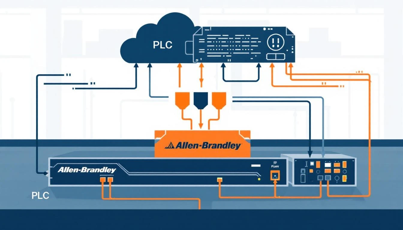
  • EtherNet/IP uses little-endian internally (Allen-Bradley heritage), but CIP encapsulation follows specific rules per data type
  • PROFINET uses big-endian for I/O data
  • OPC-UA handles byte ordering transparently — one of its few genuinely nice features

When your edge gateway reads data from a Modbus device and publishes it via MQTT to a cloud platform, you're potentially crossing three byte-ordering boundaries. Get any one of them wrong and your data is silently corrupt.

The Modbus Register Map Problem

Modbus organizes data into four register types, each accessed by a different function code:

Address RangeRegister TypeFunction CodeData DirectionAccess
0–65,535Coils (discrete outputs)FC 01Read1-bit
100,000–165,535Discrete InputsFC 02Read1-bit
300,000–365,535Input RegistersFC 04Read-only16-bit
400,000–465,535Holding RegistersFC 03Read/Write16-bit

The address ranges are a convention, not a protocol requirement. Your gateway needs to map addresses to function codes:

  • Addresses 0–65,535 → FC 01 (Read Coils)
  • Addresses 100,000–165,535 → FC 02 (Read Discrete Inputs)
  • Addresses 300,000–365,535 → FC 04 (Read Input Registers)
  • Addresses 400,000–465,535 → FC 03 (Read Holding Registers)

The actual register address sent in the Modbus PDU is the offset within the range. So address 400,100 becomes register 100 using function code 03.

Why this matters for normalization: A tag configured with address 300,800 means "read input register 800 using FC 04." A tag at address 400,520 means "read holding register 520 using FC 03." If your gateway mixes these up, it reads the wrong register type entirely — and the PLC happily returns whatever lives at that address, with no type error.

Reading Coils vs Registers: Type Coercion

When reading coils (FC 01/02), the response contains bit-packed data — each coil is a single bit. When reading registers (FC 03/04), each register is a 16-bit word.

The tricky part is mapping these raw responses to typed tag values. Consider a tag configured as uint16 that's being read from a coil address. The raw response is a single bit (0 or 1), but the tag expects a 16-bit value. Your gateway must handle this coercion:

Coil response → bool tag:     bit value directly
Coil response → uint8 tag: cast to uint8
Coil response → uint16 tag: cast to uint16
Coil response → int32 tag: cast to int32 (effectively 0 or 1)

For register responses, the mapping depends on the element count — how many consecutive registers are combined to form the value:

1 register (elem_count=1):
→ uint16: direct value
→ int16: interpret as signed
→ uint8: mask with 0xFF (lower byte)
→ bool: mask with 0xFF, then boolean

2 registers (elem_count=2):
→ uint32: combine two 16-bit registers
→ int32: interpret combined value as signed
→ float: interpret combined value as IEEE 754

The 32-Bit Register Combination Problem

Here's where manufacturers diverge and data corruption begins. A 32-bit value (integer or float) spans two consecutive 16-bit Modbus registers. But which register contains the high word?

Word Order Variants

Big-endian word order (AB CD): Register N contains the high word, register N+1 contains the low word.

Register[N]   = 0x4248    (high word)
Register[N+1] = 0x0000 (low word)
Combined = 0x42480000
As float = 50.0

Little-endian word order (CD AB): Register N contains the low word, register N+1 contains the high word.

Register[N]   = 0x0000    (low word)
Register[N+1] = 0x4248 (high word)
Combined = 0x42480000
As float = 50.0

Byte-swapped big-endian (BA DC): Each register's bytes are swapped, then combined in big-endian order.

Register[N]   = 0x4842    (swapped high)
Register[N+1] = 0x0000 (swapped low)
Combined = 0x42480000
As float = 50.0

Byte-swapped little-endian (DC BA): Each register's bytes are swapped, then combined in little-endian order.

Register[N]   = 0x0000    (swapped low)
Register[N+1] = 0x4842 (swapped high)
Combined = 0x42480000
As float = 50.0

All four combinations are found in the wild. Schneider PLCs typically use big-endian word order. Some Siemens devices use byte-swapped variants. Many Chinese-manufactured VFDs (variable frequency drives) use little-endian word order. There is no way to detect the word order automatically — you must know it from the device documentation or determine it empirically.

Practical Detection Technique

When commissioning a new device and the word order isn't documented:

  1. Find a register that should contain a known float value (like a temperature reading you can verify with a handheld thermometer)
  2. Read two consecutive registers and try all four combinations
  3. The one that produces a physically reasonable value is your word order

For example, if the device reads temperature and the registers contain 0x4220 and 0x0000:

  • AB CD: 0x42200000 = 40.0 ← probably correct if room temp
  • CD AB: 0x00004220 = 5.9×10⁻⁴¹ ← nonsense
  • BA DC: 0x20420000 = 1.6×10⁻¹⁹ ← nonsense
  • DC BA: 0x00002042 = 1.1×10⁻⁴¹ ← nonsense

IEEE 754 Floating-Point Reconstruction

Reading a float from Modbus registers requires careful reconstruction. The standard approach:

Given: Register[N] = high_word, Register[N+1] = low_word (big-endian word order)

Step 1: Combine into 32 bits
uint32 combined = (high_word << 16) | low_word

Step 2: Reinterpret as IEEE 754 float
float value = *(float*)&combined // C-style type punning
// Or use modbus_get_float() from libmodbus

The critical detail: do not cast the integer to float — that performs a numeric conversion. You need to reinterpret the same bit pattern as a float. This is the difference between getting 50.0 (correct) and getting 1110441984.0 (the integer 0x42480000 converted to float).

Common Float Pitfalls

NaN and Infinity: IEEE 754 reserves certain bit patterns for special values. If your combined registers produce 0x7FC00000, that's NaN. If you see 0x7F800000, that's positive infinity. These often appear when:

  • The sensor is disconnected (NaN)
  • The measurement is out of range (Infinity)
  • The registers are being read during a PLC scan update (race condition producing a half-updated value)

Denormalized numbers: Very small float values (< 1.175×10⁻³⁸) are "denormalized" and may lose precision. In industrial contexts, if you're seeing numbers this small, something is wrong with your byte ordering.

Zero detection: A float value of exactly 0.0 is 0x00000000. But 0x80000000 is negative zero (-0.0). Both compare equal in standard float comparison, but the bit patterns are different. If you're doing bitwise comparison for change detection, be aware of this edge case.

Scaling Factors: From Raw to Engineering Units

Many industrial devices don't transmit floating-point values. Instead, they send raw integers that must be scaled to engineering units. This is especially common with:

  • Temperature transmitters (raw: 0–4000 → scaled: 0–100°C)
  • Pressure sensors (raw: 0–65535 → scaled: 0–250 PSI)
  • Flow meters (raw: counts/second → scaled: gallons/minute)

Linear Scaling

The most common pattern is linear scaling with two coefficients:

engineering_value = (raw_value × k1) / k2

Where k1 and k2 are integer scaling coefficients defined in the tag configuration. This avoids floating-point math on resource-constrained edge devices.

Examples:

  • Temperature: k1=1, k2=10 → raw 1675 becomes 167.5°C
  • Pressure: k1=250, k2=65535 → raw 32768 becomes 125.0 PSI
  • RPM: k1=1, k2=1 → raw value is direct (no scaling)

Important: k2 must never be zero. Always validate configuration before applying scaling — a division-by-zero in an edge gateway's main loop crashes the entire data acquisition pipeline.

Bit Extraction (Calculated Tags)

Some devices pack multiple boolean values into a single register. A 16-bit "status word" might contain:

Bit 0: Motor Running
Bit 1: Fault Active
Bit 2: High Temperature
Bit 3: Low Pressure
Bits 4-7: Operating Mode
Bits 8-15: Reserved

Extracting individual values requires bitwise operations:

motor_running = (status_word >> 0) & 0x01    // shift=0, mask=1
fault_active = (status_word >> 1) & 0x01 // shift=1, mask=1
op_mode = (status_word >> 4) & 0x0F // shift=4, mask=15

In a well-designed edge gateway, these "calculated tags" are defined as children of the parent register tag. When the parent register value changes, the gateway automatically recalculates all child tags and delivers their values. This eliminates redundant register reads — you read the status word once and derive multiple data points.

Dependent Tag Chains

Beyond simple bit extraction, production systems use dependent tag chains: when tag A changes, immediately read tags B, C, and D regardless of their normal polling interval.

Example: When machine_state transitions from 0 (IDLE) to 1 (RUNNING), immediately read:

  • Current speed setpoint
  • Actual motor RPM
  • Material temperature
  • Batch counter

This captures the complete state snapshot at the moment of transition, which is far more valuable than catching each value at their independent polling intervals (where you might see the new speed 5 seconds after the state change).

The key architectural insight: tag dependencies form a directed acyclic graph. The edge gateway must traverse this graph depth-first on each parent change, reading and delivering dependent tags within the same batch timestamp for temporal coherence.

Binary Serialization for Bandwidth Efficiency

Once values are normalized, they need to be serialized for transport. Two common formats:

JSON (Human-Readable)

{
"groups": [{
"ts": 1709510400,
"device_type": 1011,
"serial_number": 12345,
"values": [
{"id": 1, "values": [167.5]},
{"id": 2, "values": [true]},
{"id": 3, "values": [1250, 1248, 1251, 1249, 1250, 1252]}
]
}]
}

Binary (Bandwidth-Optimized)

A compact binary format packs the same data into roughly 20–30% of the JSON size:

Byte 0:     0xF7 (frame identifier)
Bytes 1-4: Number of groups (uint32, big-endian)

Per group:
4 bytes: Timestamp (uint32)
2 bytes: Device type (uint16)
4 bytes: Serial number (uint32)
4 bytes: Number of values (uint32)

Per value:
2 bytes: Tag ID (uint16)
1 byte: Status (0x00 = OK, else error code)
If status == OK:
1 byte: Array size (number of elements)
1 byte: Element size (1, 2, or 4 bytes)
N bytes: Packed values, each big-endian

Value packing examples:

bool:   true  → 0x01           (1 byte)
bool: false → 0x00 (1 byte)
int16: 55 → 0x00 0x37 (2 bytes, big-endian)
int16: -55 → 0xFF 0xC9 (2 bytes, two's complement)
uint16: 32768 → 0x80 0x00
int32: 55 → 0x00 0x00 0x00 0x37
float: 1.55 → 0x3F 0xC6 0x66 0x66 (IEEE 754)
float: -1.55 → 0xBF 0xC6 0x66 0x66

Note the byte ordering in the serialization format: values are packed big-endian (MSB first) regardless of the source device's native byte ordering. The edge gateway normalizes byte order during serialization, so the cloud consumer never needs to worry about endianness.

Register Grouping and Read Optimization

Modbus allows reading up to 125 consecutive registers in a single request (FC 03/04). A naive implementation sends one request per tag — reading 50 tags requires 50 round trips, each with its own Modbus frame overhead and inter-frame delay.

A well-optimized gateway groups tags by:

  1. Same function code — Tags addressed at 400,100 and 300,100 cannot be grouped (different FC)
  2. Contiguous addresses — Tags at addresses 400,100 and 400,101 can be read in one request
  3. Same polling interval — Tags with different intervals should be in separate groups to avoid reading slow-interval tags too frequently
  4. Maximum register count — Cap at ~50 registers per request to stay well within Modbus limits and avoid timeout issues with slower devices

The algorithm: sort tags by address, then walk the sorted list. Start a new group when:

  • The function code changes
  • The address is not contiguous with the previous tag
  • The polling interval differs
  • The accumulated register count exceeds the maximum

After each group read, insert a brief pause (50ms is typical) before the next read. This prevents overwhelming slow Modbus devices that need time between transactions to process their internal scan.

Change Detection and Comparison

For bandwidth-constrained deployments (cellular, satellite, LoRaWAN backhaul), sending every value on every read cycle is wasteful. Implement value comparison:

On each tag read:
if (tag.compare_enabled):
if (new_value == last_value) AND (status unchanged):
skip delivery
else:
deliver value
update last_value
else:
always deliver

The comparison must be type-aware:

  • Integer types: Direct bitwise comparison (uint_value != last_uint_value)
  • Float types: Bitwise comparison, NOT approximate comparison. In industrial contexts, if the bits didn't change, the value didn't change. Using epsilon-based comparison would miss relevant changes while potentially false-triggering on noise.
  • Boolean types: Direct comparison

Periodic forced delivery: Even with comparison enabled, force-deliver all tag values once per hour. This ensures the cloud state eventually converges with reality, even if a value change was missed during a brief network outage.

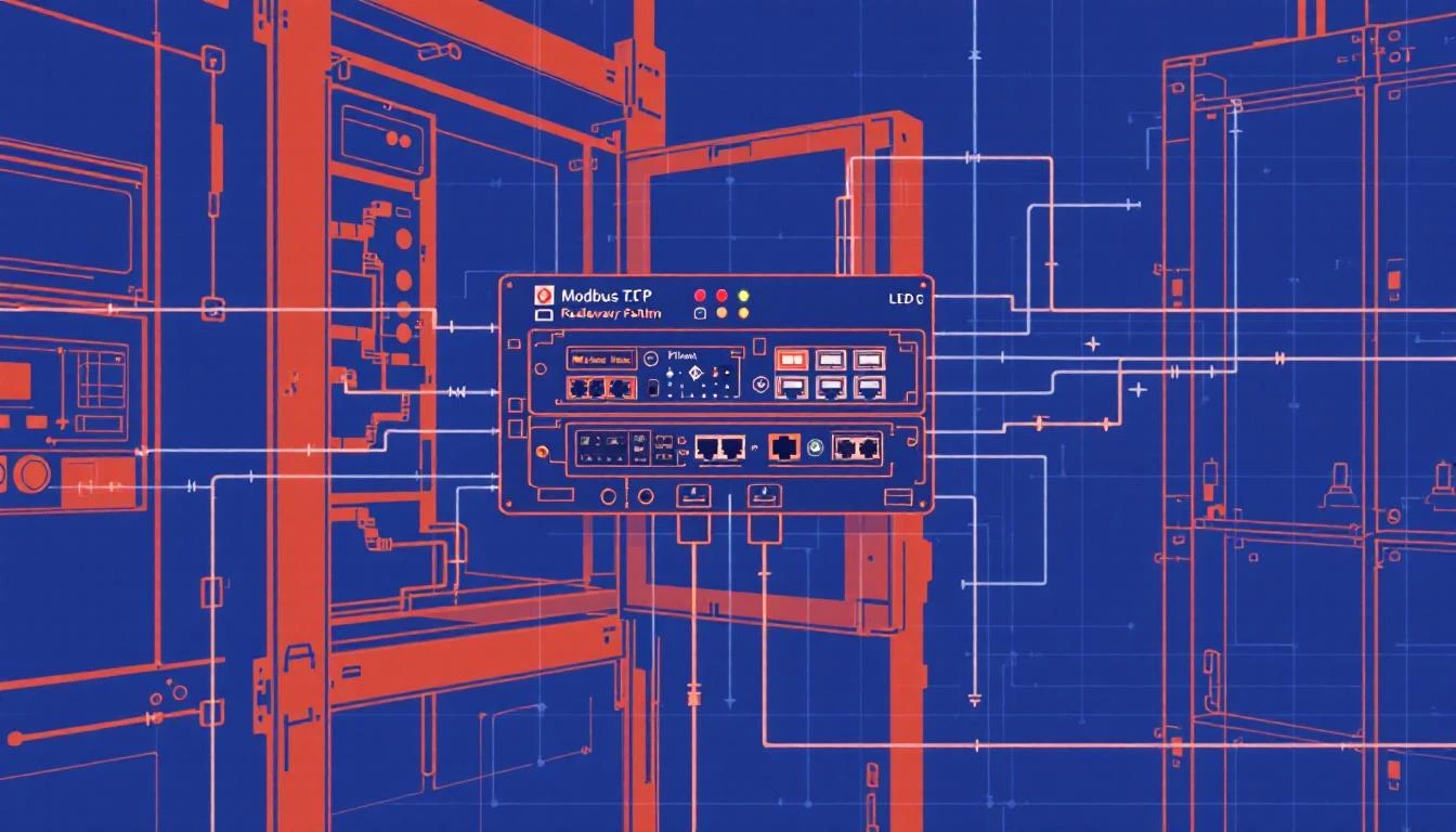
Handling Modbus RTU vs TCP

The normalization logic is identical for Modbus RTU (serial) and Modbus TCP (Ethernet). The differences are all in the transport layer:

ParameterModbus RTUModbus TCP
PhysicalRS-485 serialEthernet
ConnectionSerial port openTCP socket connect
AddressingSlave address (1-247)IP:port (default 502)
FramingCRC-16MBAP header
TimingInter-character timeout mattersTCP handles retransmission
Baud rate9600–115200 typicalN/A (Ethernet speed)
Response timeout400ms typicalShorter (network dependent)

RTU-Specific Configuration

For Modbus RTU, the serial link parameters must match the device exactly:

Baud rate:       9600 (most common) or 19200, 38400, 115200
Parity: None, Even, or Odd
Data bits: 8 (almost always)
Stop bits: 1 or 2
Slave address: 1-247
Byte timeout: 50ms (time between bytes in a frame)
Response timeout: 400ms (time to wait for a response)

Critical RTU detail: Always flush the serial buffer before starting a new transaction. Stale bytes in the receive buffer from a previous timed-out response will corrupt the current response parsing. This is the number one cause of intermittent "bad CRC" errors on Modbus RTU links.

Error Handling That Matters

When a Modbus read fails, the error code tells you what went wrong:

errnoMeaningRecovery Action
ETIMEDOUTDevice didn't respondRetry 2x, then mark link DOWN
ECONNRESETConnection droppedClose + reconnect
ECONNREFUSEDDevice rejected connectionCheck IP/port, wait before retry
EPIPEBroken pipeClose + reconnect
EBADFBad file descriptorSocket is dead, full reinit

On any of these errors, the correct response is: flush the connection, close it, mark the device link state as DOWN, and attempt reconnection on the next cycle. Don't try to send more data on a dead connection — it will fail faster than you can log it.

Deliver error status alongside the tag. When a tag read fails, don't silently drop the data point. Deliver the tag ID with a non-zero status code and no value data. This lets the cloud platform distinguish between "the sensor reads 0" and "we couldn't reach the sensor." They're very different situations.

How machineCDN Handles Data Normalization

machineCDN's edge runtime performs all normalization at the device boundary — byte order conversion, type coercion, bit extraction, scaling, and comparison — before data touches the network. The binary serialization format described above is the actual wire format used between edge gateways and the machineCDN cloud, achieving typical compression ratios of 3–5x versus JSON while maintaining full type fidelity.

For plant engineers, this means you configure tags with their register addresses, data types, and scaling factors. The platform handles the byte-level mechanics — you never need to manually swap words, reconstruct floats, or debug endianness issues. Tag values arrive in the cloud as properly typed, correctly scaled engineering units, ready for dashboards, analytics, and alerting.

Checklist: Commissioning a New Device

When connecting a new Modbus device to your IIoT platform:

  1. Identify the register map — Get the manufacturer's documentation. Don't guess addresses.
  2. Determine the word order — Read a known float value and try all four combinations.
  3. Verify function codes — Confirm which registers use FC 03 vs FC 04.
  4. Check the slave address — RTU only; confirm via device configuration panel.
  5. Set appropriate timeouts — 50ms byte timeout, 400ms response timeout for RTU; 2000ms for TCP.
  6. Read one tag at a time first — Validate each tag independently before grouping.
  7. Compare with HMI values — Cross-reference your gateway's readings against the device's local display.
  8. Enable comparison selectively — For status bits and slow-changing values only. Disable for process variables during commissioning.
  9. Monitor for -32 / timeout errors — Persistent errors indicate wiring, addressing, or timing issues.
  10. Document everything — Future you will not remember why tag 0x1A uses elem_count=2 with k1=10 and k2=100.

Conclusion

Data normalization is the unglamorous foundation of every working IIoT system. When it works, nobody notices. When it fails, your dashboards show nonsense and operators lose trust in the platform.

The key principles:

  • Know your byte order — and document it per device
  • Match element size to data type — a 4-byte read on a 2-byte register reads adjacent memory
  • Use bitwise comparison for floats — not epsilon
  • Batch and serialize efficiently — binary beats JSON for bandwidth-constrained links
  • Group contiguous registers — reduce Modbus round trips by 5–10x
  • Always deliver error status — silent data drops are worse than explicit failures

Get these right at the edge, and every layer above — time-series databases, dashboards, ML models, alerting — inherits clean, trustworthy data. Get them wrong, and no amount of cloud processing can fix values that were corrupted before they left the factory floor.

Why Most Manufacturing AI Projects Stall After the Pilot Phase (And the 5 Fixes That Actually Work)

· 11 min read
MachineCDN Team
Industrial IoT Experts

The pilot worked beautifully. Your AI model predicted bearing failures on Line 3 with 94% accuracy. The CEO saw the demo. The board heard about "digital transformation." Budget was approved for a plant-wide rollout.

That was eighteen months ago. The model still runs on Line 3. Maintenance still uses clipboards everywhere else. The data scientist who built the pilot left for a fintech startup. And nobody can explain why a model that worked perfectly on one line won't work on the other seven.

If this sounds familiar, you're not alone. According to a McKinsey survey on AI in manufacturing, 87% of manufacturing AI projects never make it past the pilot phase. Not because the AI doesn't work — but because the organizational, data, and infrastructure challenges of scaling from one line to a full plant were never addressed.

The AI isn't the problem. The pilot model is the problem.

The Convergence of MES and IIoT: Why Traditional Manufacturing Execution Systems Are Being Disrupted

· 10 min read
MachineCDN Team
Industrial IoT Experts

The manufacturing execution system (MES) market hit $16.7 billion in 2025. By 2030, analysts project $28.3 billion. And yet, the most interesting thing happening in manufacturing software isn't MES growing — it's MES being absorbed.

IIoT platforms are eating MES functionality from the bottom up. What started as simple machine monitoring (connect a sensor, see a dashboard) has expanded to include OEE tracking, downtime analysis, quality management, production scheduling, and work order management — the traditional domain of enterprise MES.

Meanwhile, MES vendors are adding IIoT features — edge connectivity, real-time machine data, predictive analytics — from the top down. The two categories are converging, and the result is a fundamental disruption of how manufacturers think about their factory software stack.

If your plant is running a 10-year-old MES — or worse, if you're about to sign a 7-figure MES contract — this convergence matters to you. Here's what's actually happening and what to do about it.

Modbus RTU Serial Link Diagnostics: Timeout Tuning, Error Recovery, and Fieldbus Troubleshooting [2026]

· 12 min read

If you've ever stared at a Modbus RTU link that mostly works — dropping one request out of fifty, returning CRC errors at 2 AM, or silently losing a slave device after a power blip — you know that "mostly works" is the most dangerous state in industrial automation.

Modbus TCP gets all the attention in modern IIoT discussions, but the factory floor still runs on RS-485 serial. Chillers, temperature controllers, VFDs, auxiliary equipment — an enormous installed base of devices still speaks Modbus RTU over twisted-pair wiring. Getting that serial link right is the difference between a monitoring system that earns trust and one that gets unplugged.

This guide covers the diagnostic techniques and configuration strategies that separate a bulletproof Modbus RTU deployment from a frustrating one.

Modbus TCP Gateway Failover: Building Redundant PLC Communication for Manufacturing [2026]

· 14 min read

Modbus TCP gateway failover architecture

Modbus TCP remains the most widely deployed industrial protocol in manufacturing. Despite being a 1979 design extended to Ethernet in 1999, its simplicity — request/response over TCP, 16-bit registers, four function codes that cover 90% of use cases — makes it the lowest common denominator that virtually every PLC, VFD, and sensor hub supports.

But simplicity has a cost: Modbus TCP has zero built-in redundancy. No heartbeats. No automatic reconnection. No session recovery. When the TCP connection drops — and in a factory environment with electrical noise, cable vibrations, and switch reboots, it will drop — your data collection goes dark until someone manually restarts the gateway or the application logic handles recovery.

This guide covers the architecture patterns for building resilient Modbus TCP gateways that maintain data continuity through link failures, PLC reboots, and network partitions.

Understanding Why Modbus TCP Connections Fail

Before designing failover, you need to understand the failure modes. In a year of operating Modbus TCP gateways across manufacturing floors, you'll encounter all of these:

Failure Mode 1: TCP Connection Reset (ECONNRESET)

The PLC or an intermediate switch drops the TCP connection. Common causes:

  • PLC firmware update or watchdog reboot
  • Switch port flap (cable vibration, loose connector)
  • PLC connection limit exceeded (most support 6-16 simultaneous TCP connections)
  • Network switch spanning tree reconvergence (can take 30-50 seconds on older managed switches)

Detection time: Immediate — the next modbus_read_registers() call returns ECONNRESET.

Failure Mode 2: Connection Timeout (ETIMEDOUT)

The PLC stops responding but doesn't close the connection. The TCP socket remains open, but reads time out. Common causes:

  • PLC CPU overloaded (complex ladder logic consuming all scan cycles)
  • Network congestion (broadcast storms, misconfigured VLANs)
  • IP conflict (another device grabbed the PLC's address)
  • PLC in STOP mode (program halted, communication stack still partially active)

Detection time: Your configured response timeout (typically 500ms-2s) per read operation. For a 100-tag poll cycle, a full timeout can mean 50-200 seconds of dead time before you confirm the link is down.

Failure Mode 3: Connection Refused (ECONNREFUSED)

The PLC's TCP stack is active but Modbus is not. Common causes:

  • PLC in bootloader mode after firmware flash
  • Modbus TCP server disabled in PLC configuration
  • Firewall rule change on managed switch blocking port 502

Detection time: Immediate on the next connection attempt.

Failure Mode 4: Silent Failure (EPIPE/EBADF)

The connection appears open from the gateway's perspective, but the PLC has already closed it. The first write or read on a stale socket triggers EPIPE or EBADF. This happens when:

  • PLC reboots cleanly but the gateway missed the FIN packet (common with UDP-accelerated switches)
  • OS socket cleanup runs asynchronously

Detection time: Only on the next read/write attempt — could be seconds to minutes if polling intervals are long.

The Connection Recovery State Machine

A resilient Modbus TCP gateway implements a state machine with five states:

                    ┌─────────────┐
│ CONNECTING │
│ (backoff) │
└──────┬──────┘
│ modbus_connect() success
┌──────▼──────┐
┌─────│ CONNECTED │─────┐
│ │ (polling) │ │
│ └──────┬──────┘ │
│ │ │
timeout/error link_state=1 read error
│ │ │
┌────────▼───┐ ┌─────▼─────┐ ┌──▼──────────┐
│ RECONNECT │ │ READING │ │ LINK_DOWN │
│ (flush + │ │ (normal) │ │ (notify + │
│ close) │ │ │ │ reconnect) │
└────────┬───┘ └───────────┘ └──┬──────────┘
│ │
└────────────────────────┘
close + backoff

Key Implementation Details

1. Always close before reconnecting. A stale Modbus context will leak file descriptors and eventually exhaust the OS socket table. When any error occurs in the ETIMEDOUT/ECONNRESET/EPIPE/EBADF family, the correct sequence is:

modbus_flush(context)   → drain pending data
modbus_close(context) → close the TCP socket
sleep(backoff_ms) → prevent reconnection storms
modbus_connect(context) → establish new connection

Never call modbus_connect() on a context that hasn't been closed first. The libmodbus library doesn't handle this gracefully — you'll get zombie sockets.

2. Implement exponential backoff with a ceiling. After a connection failure, don't retry immediately — the PLC may be rebooting and needs time. A practical backoff schedule:

AttemptDelayCumulative Time
11 second1s
22 seconds3s
34 seconds7s
48 seconds15s
5+10 seconds (ceiling)25s+

The 10-second ceiling is important — you don't want the backoff growing to minutes. PLC reboots typically complete in 15-45 seconds. A 10-second retry interval means you'll reconnect within one retry cycle after the PLC comes back.

3. Flush serial buffers for Modbus RTU. If your gateway also supports Modbus RTU (serial), always call modbus_flush() before reading after a reconnection. Serial buffers can contain stale response fragments from before the disconnection, and these will corrupt the first read's response parsing.

4. Track link state as a first-class data point. Don't just log connection status — deliver it to the cloud alongside your tag data. A special "link state" tag (boolean: 0 = disconnected, 1 = connected) transmitted immediately (not batched) gives operators real-time visibility into gateway health. When the link transitions from 1→0, send a notification. When it transitions from 0→1, force-read all tags to establish current values.

Register Grouping: Minimizing Round Trips

Modbus TCP's request/response model means each read operation incurs a full TCP round trip (~0.5-5ms on a local network, 50-200ms over cellular). Reading 100 individual registers one at a time takes 100 round trips — potentially 500ms on a good day.

The optimization is contiguous register grouping — instead of reading registers one at a time, read blocks of contiguous registers in a single request.

The Grouping Algorithm

Given a sorted list of register addresses to read, the gateway walks through them and groups contiguous registers that meet three criteria:

  1. Same function code — you can't mix input registers (FC 4, 3xxxxx) with holding registers (FC 3, 4xxxxx) in one request
  2. Contiguous addresses — register N+1 immediately follows register N (with appropriate gaps filled)
  3. Same polling interval — don't group a 1-second alarm tag with a 60-second temperature tag
  4. Maximum register count ≤ 50 — while Modbus allows up to 125 registers per read, keeping requests under 50 registers (~100 bytes) prevents fragmentation issues on constrained networks and limits the blast radius of a single failed read

Example: Optimized vs Naive Polling

Consider a chiller with 10 compressor circuits, each reporting 16 process variables:

Naive approach: 160 individual reads = 160 round trips

Read register 300003 → 1 register  (CQT1 Condenser Inlet Temp)
Read register 300004 → 1 register (CQT1 Approach Temp)
Read register 300005 → 1 register (CQT1 Chill In Temp)
...
Read register 300016 → 1 register (CQT1 Superheat Temp)

Grouped approach: Registers 300003-300018 are contiguous, same function code (FC 4), same interval (60s)

Read registers 300003 → 16 registers (all CQT1 process data in ONE request)
Read registers 300350 → 16 registers (all CQT2 process data in ONE request)
...

Result: 160 round trips → 10 round trips. On a 2ms RTT network, that's 320ms → 20ms.

Handling Non-Contiguous Gaps

Real PLC register maps aren't perfectly contiguous. The chiller above has CQT1 data at registers 300003-300018 and CQT2 data starting at 300350 — a gap of 332 registers. Don't try to read 300003-300695 in one request to "fill the gap" — you'll read hundreds of irrelevant registers and waste bandwidth.

Instead, break at non-contiguous boundaries:

Group 1: 300003-300018  (16 registers, CQT1 process data)
Group 2: 300022-300023 (2 registers, CQT1 alarm bits)
Group 3: 300038-300043 (6 registers, CQT1 expansion + version)
Group 4: 300193-300194 (2 registers, CQT1 status words)
Group 5: 300260-300278 (19 registers, CQT2-10 alarm bits)
Group 6: 300350-300366 (17 registers, CQT2-3 temperatures)
...

The 50ms Inter-Read Delay

Between consecutive Modbus read requests, insert a 50ms delay. This sounds counterintuitive — why slow down? — but it serves two purposes:

  1. PLC scan cycle breathing room. Many PLCs process Modbus requests in their communication interrupt, which competes with the main scan cycle. Rapid-fire requests can extend the scan cycle, triggering watchdog timeouts on safety-critical programs.

  2. TCP congestion avoidance. On constrained networks (especially cellular gateways), bursting 50 reads in 100ms can overflow buffers. The 50ms spacing distributes the load evenly.

Dual-Path Failover Architecture

For mission-critical data collection (pharmaceutical batch records, automotive quality traceability), a single gateway represents a single point of failure. The dual-path architecture uses two independent gateways polling the same PLC:

Architecture

                    ┌──────────┐
│ PLC │
│ (Modbus) │
└──┬───┬──┘
│ │
Port 502 │ │ Port 502
│ │
┌────────▼┐ ┌▼────────┐
│Gateway A│ │Gateway B│
│(Primary)│ │(Standby)│
└────┬────┘ └────┬────┘
│ │
▼ ▼
┌────────────────────┐
│ MQTT Broker │
│ (cloud/edge) │
└────────────────────┘

Active/Standby vs Active/Active

Active/Standby: Gateway A polls the PLC. Gateway B monitors A's heartbeat (via MQTT LWT or a shared health topic). If A goes silent for >30 seconds, B starts polling. When A recovers, it checks B's status and either resumes as primary or remains standby.

  • Pro: Only one gateway reads from the PLC, respecting the PLC's connection limit
  • Con: 30-second failover gap

Active/Active: Both gateways poll the PLC simultaneously. The cloud platform deduplicates data based on timestamps and device serial numbers. If one gateway fails, the other's data is already flowing.

  • Pro: Zero-downtime failover, no coordination needed
  • Con: Doubles PLC connection count and network traffic. Most PLCs support this (6-16 connections), but verify.

Recommendation: Active/Active with cloud-side deduplication. The PLC connection overhead is negligible compared to the operational cost of a 30-second data gap. Cloud-side deduplication is trivial — tag ID + timestamp + device serial number provides a natural composite key.

Store-and-Forward: Surviving Cloud Disconnections

Gateway-to-PLC failover handles half the problem. The other half is cloud connectivity — cellular links drop, VPN tunnels restart, and MQTT brokers undergo maintenance. During these outages, the gateway must buffer data locally and forward it when connectivity returns.

The Paged Ring Buffer

A production-grade store-and-forward buffer uses a paged ring buffer — pre-allocated memory divided into fixed-size pages, with separate write and read pointers:

┌──────────┐
│ Page 0 │ ← read_pointer (next to transmit)
│ [data] │
├──────────┤
│ Page 1 │
│ [data] │
├──────────┤
│ Page 2 │ ← write_pointer (next to fill)
│ [empty] │
├──────────┤
│ Page 3 │
│ [empty] │
└──────────┘

When the MQTT connection is healthy:

  1. Tag data is written to the current work page
  2. When the page fills, it moves to the "used" queue
  3. The buffer transmits the oldest used page to MQTT (QoS 1 for delivery confirmation)
  4. On publish acknowledgment, the page moves to the "free" queue

When the MQTT connection drops:

  1. Tag data continues writing to pages (the PLC doesn't stop producing data)
  2. Used pages accumulate in the queue
  3. If the queue fills, the oldest used page is recycled as a work page — accepting data loss of the oldest data to preserve the newest

This design guarantees:

  • Constant memory usage — no dynamic allocation on an embedded device
  • Graceful degradation — oldest data is sacrificed first
  • Thread safety — mutex-protected page transitions prevent race conditions between the reading thread (PLC poller) and writing thread (MQTT publisher)

Sizing the Buffer

Buffer size depends on your data rate and expected maximum outage duration:

buffer_size = data_rate_bytes_per_second × max_outage_seconds × 1.2 (overhead)

For a typical deployment:

  • 100 tags × 4 bytes/value = 400 bytes per poll cycle
  • 1 poll per second = 400 bytes/second
  • Binary encoding with batch overhead: ~500 bytes/second
  • Target 4 hours of offline buffering: 500 × 14,400 = 7.2MB

With 512KB pages, that's ~14 pages. Allocate 16 pages (minimum 3 needed for operation: one writing, one transmitting, one free) for an 8MB buffer.

Binary vs JSON Encoding for Buffered Data

JSON is wasteful for buffered data. The same 100-tag reading:

  • JSON: {"groups":[{"ts":1709500800,"device_type":1018,"serial_number":23456,"values":[{"id":1,"values":[245]},{"id":2,"values":[312]},...]}]} → ~2KB
  • Binary: Header (0xF7 + group count + timestamp + device info) + packed tag values → ~500 bytes

Binary encoding uses a compact format:

[0xF7] [num_groups:4] [timestamp:4] [device_type:2] [serial_num:4] 
[num_values:4] [tag_id:2] [status:1] [value_count:1] [value_size:1] [values...]

Over a cellular connection billing at $5/GB, the 4× bandwidth savings of binary encoding pays for itself within days on a busy gateway.

Alarm Tag Priority: Batched vs Immediate Delivery

Not all tags are created equal. A temperature reading that's 0.1°C different from the last poll can wait for the next batch. An alarm bit that just flipped from 0 to 1 cannot.

The gateway should support two delivery modes per tag:

Batched Delivery (Default)

Tags are accumulated in the batch buffer and delivered on the batch timeout (typically 5-30 seconds) or batch size limit (typically 10-500KB). This is efficient for process variables that change slowly.

Configuration:

{
"name": "Tank Temperature",
"id": 1,
"addr": 300202,
"type": "int16",
"interval": 60,
"compare": false
}

Immediate Delivery (do_not_batch)

Tags bypass the batch buffer entirely. When the value changes, a single-value batch is created, serialized, and pushed to the output buffer immediately. This is essential for:

  • Alarm words — operators need sub-second alarm notification
  • Machine state transitions — running/stopped/faulted changes trigger downstream actions
  • Safety interlocks — any safety-relevant state change must be delivered without batching delay

Configuration:

{
"name": "CQT 1 Alarm Bits 1",
"id": 163,
"addr": 300022,
"type": "uint16",
"interval": 1,
"compare": true,
"do_not_batch": true
}

The compare: true flag is critical for immediate-delivery tags — without it, the gateway would transmit on every read cycle (every 1 second), flooding the network. With comparison enabled, the gateway only transmits when the alarm word actually changes — zero bandwidth during normal operation, instant delivery when an alarm fires.

Calculated Tags: Extracting Bit-Level Alarms from PLC Words

Many PLCs pack multiple alarm states into a single 16-bit register. Bit 0 might indicate "high temperature," bit 1 "low flow," bit 2 "compressor fault," etc. Rather than requiring the cloud platform to perform bitwise decoding, a production gateway extracts individual bits and delivers them as separate boolean tags.

The extraction uses shift-and-mask arithmetic:

alarm_word = 0xA5 = 10100101 in binary

bit_0 = (alarm_word >> 0) & 0x01 = 1 → "High Temperature" = TRUE
bit_1 = (alarm_word >> 1) & 0x01 = 0 → "Low Flow" = FALSE
bit_2 = (alarm_word >> 2) & 0x01 = 1 → "Compressor Fault" = TRUE
...

These calculated tags are defined as children of the parent alarm word. When the parent tag changes value (detected by the compare flag), all child calculated tags are re-evaluated and delivered. If the parent doesn't change, no child processing occurs — zero CPU overhead during steady state.

This architecture keeps the PLC configuration simple (one alarm word per circuit) while giving cloud consumers individual, addressable alarm signals.

Putting It All Together: A Production Gateway Checklist

Before deploying a Modbus TCP gateway to production, verify:

  • Connection recovery handles all five error codes (ETIMEDOUT, ECONNRESET, ECONNREFUSED, EPIPE, EBADF)
  • Exponential backoff with 10-second ceiling prevents reconnection storms
  • Link state is delivered as a first-class tag (not just logged)
  • Register grouping batches contiguous same-function-code registers (max 50 per read)
  • 50ms inter-read delay protects PLC scan cycle integrity
  • Store-and-forward buffer sized for target offline duration
  • Binary encoding used for buffered data (not JSON)
  • Alarm tags configured with compare: true and immediate delivery
  • Calculated tags extract individual bits from alarm words
  • Force-read on reconnection ensures fresh values after any link recovery
  • Hourly full re-read resets all "read once" flags to catch any drift

machineCDN and Modbus TCP

machineCDN's edge gateway implements these patterns natively — connection state management, contiguous register grouping, binary batch encoding, paged ring buffers, and calculated alarm tags — so that plant engineers can focus on which tags to monitor rather than how to keep the data flowing. The gateway's JSON-based tag configuration maps directly to the PLC's register map, and the dual-format delivery system (binary for efficiency, JSON for interoperability) adapts to whatever network path is available.

For manufacturing teams running Modbus TCP equipment — from chillers and dryers to injection molding machines and conveying systems — getting the gateway layer right is the difference between a monitoring system that works in the lab and one that survives a year on the factory floor.


Building a Modbus TCP monitoring system? machineCDN handles protocol translation, buffering, and cloud delivery for manufacturing equipment — so your data keeps flowing even when your network doesn't.